Category: Profilometry | Texture and Grain

Stent Coating Adhesion and Delamination Analysis Using Nano Scratch Testing

Application Note | Stent Coating Adhesion Testing

Stent Coating Adhesion and Delamination Analysis Using Nano Scratch Testing

Quantifying Coating Failure and Adhesion Performance on Drug-Eluting Stents

Research & Experimental Testing

Duanjie Li, PhD

Visual Design & Editorial

Andrew Shore

Introduction

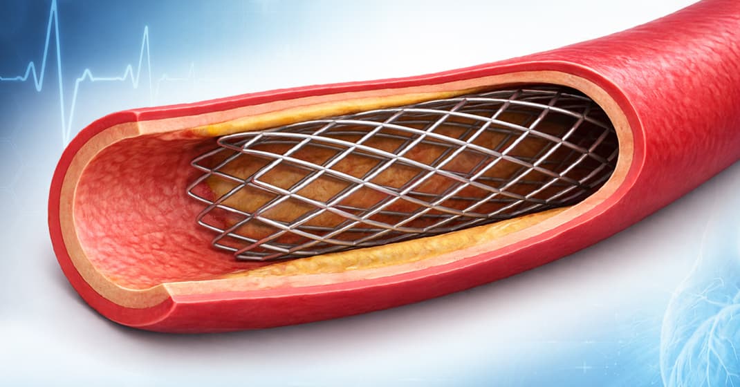
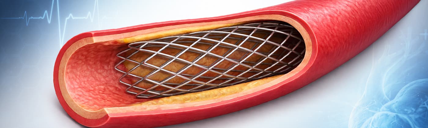
Blood is carried through arteries from the heart to the rest of the body. Any weakening or blockage of these vessels can pose significant health risks and may become life-threatening. A stent is a small mesh tube inserted into the lumen of a blood vessel to treat narrowed or weakened arteries. Stent implantation is now a widely used procedure to support the arterial wall and restore blood flowᶦ.

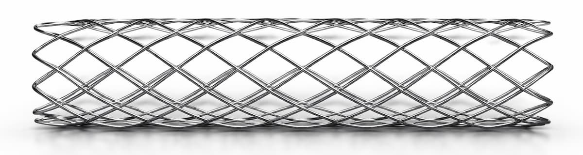
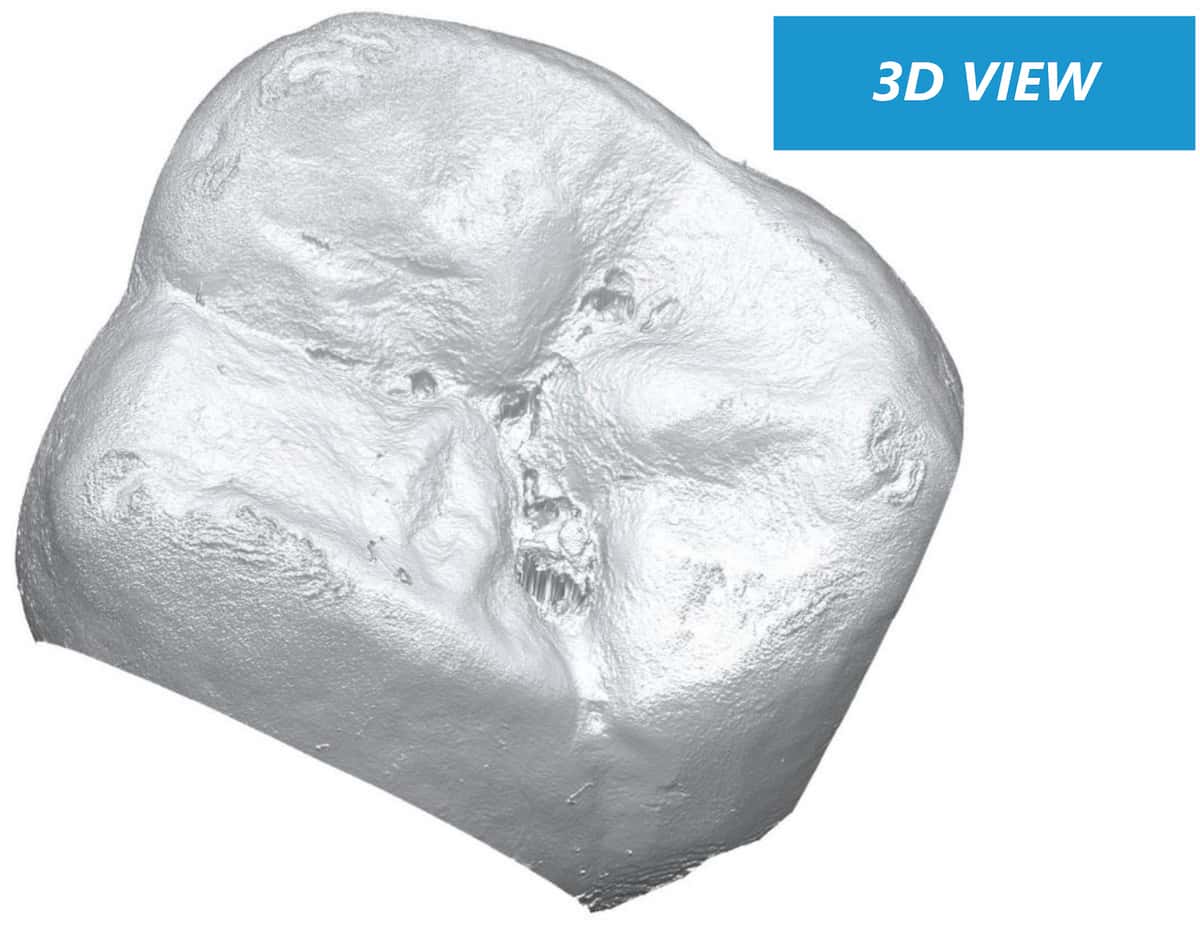
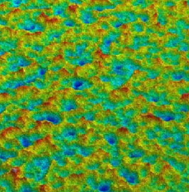
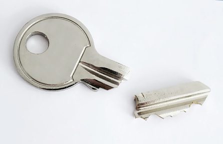
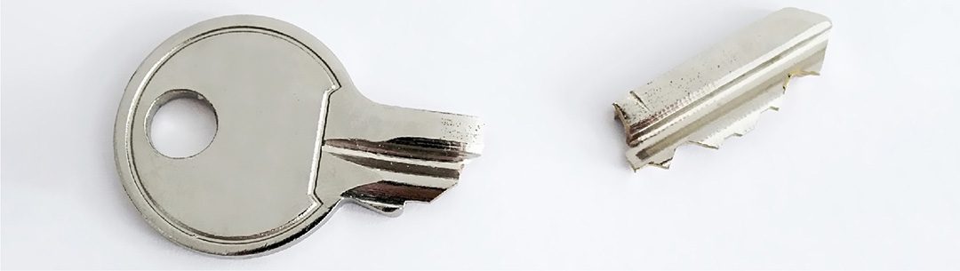
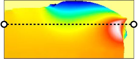
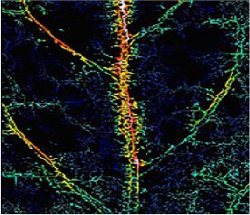
Metal stent mesh geometry illustrating the structural complexity of vascular implant design.

Why coating adhesion matters in drug-eluting stents

Drug-eluting stents represent a major advancement in stent technology. They incorporate a biodegradable, biocompatible polymer coating that enables controlled drug release at the arterial site, helping to inhibit intimal thickening and reduce the risk of restenosisᶦᶦ.

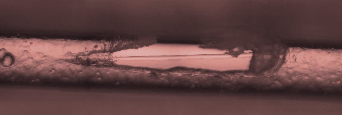
A critical concern in these systems is the delamination of the polymer coating from the metallic stent substrate. This coating carries the drug-eluting layer, and its adhesion directly impacts device performance and reliability.

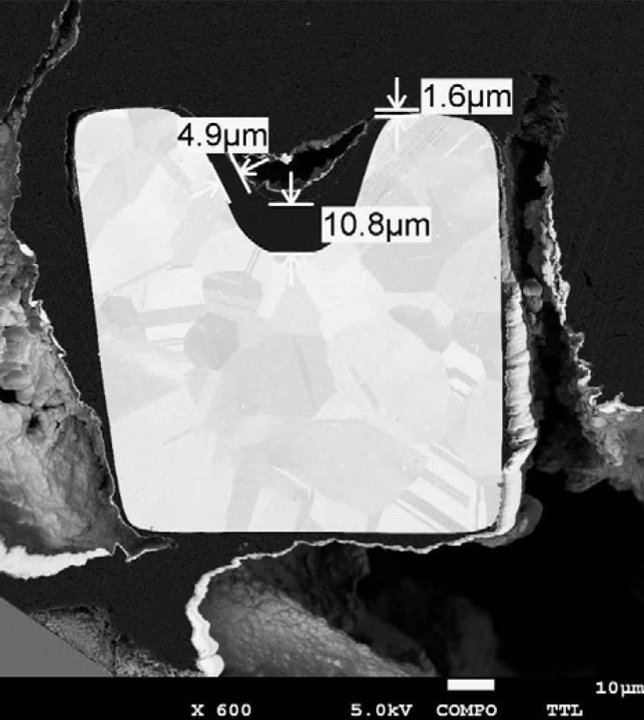
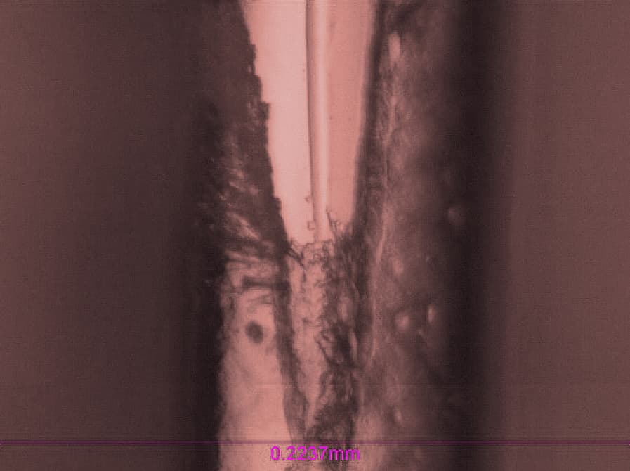
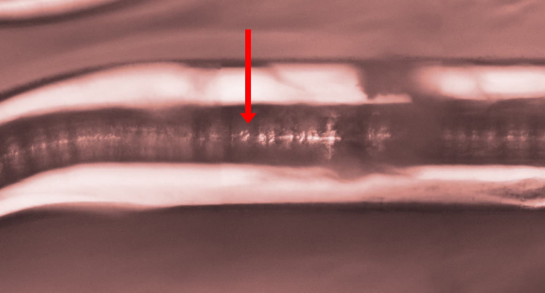
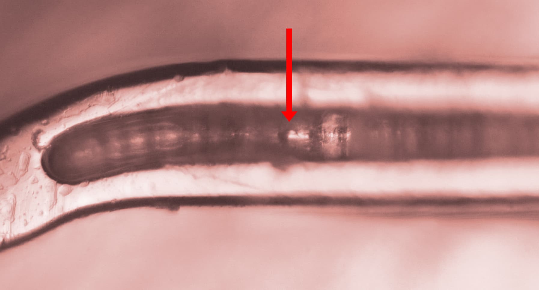
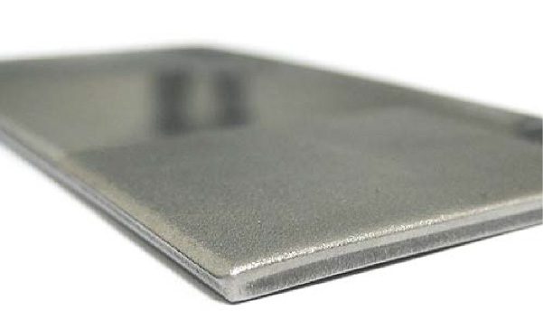
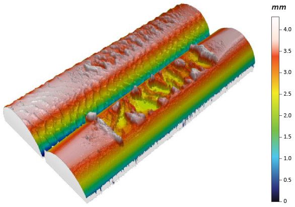
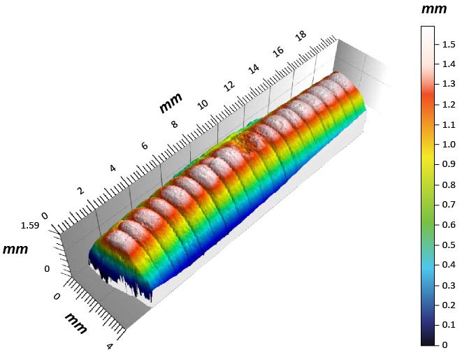
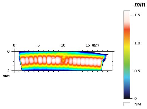
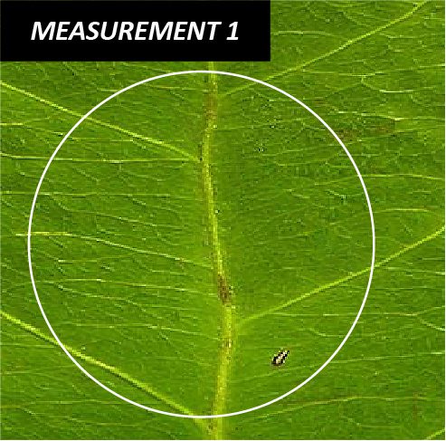
To improve coating adhesion, stents are often designed with complex geometries. In this study, the polymer coating is located at the bottom of grooves within the stent mesh. This configuration presents a significant challenge for adhesion measurement.

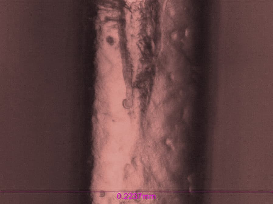
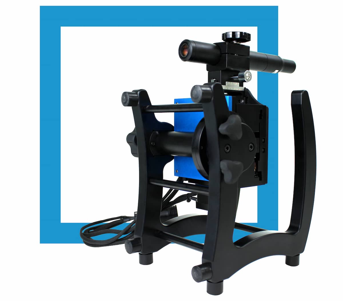
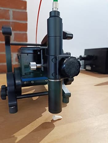
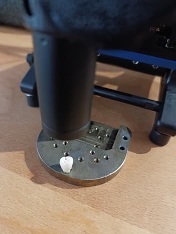
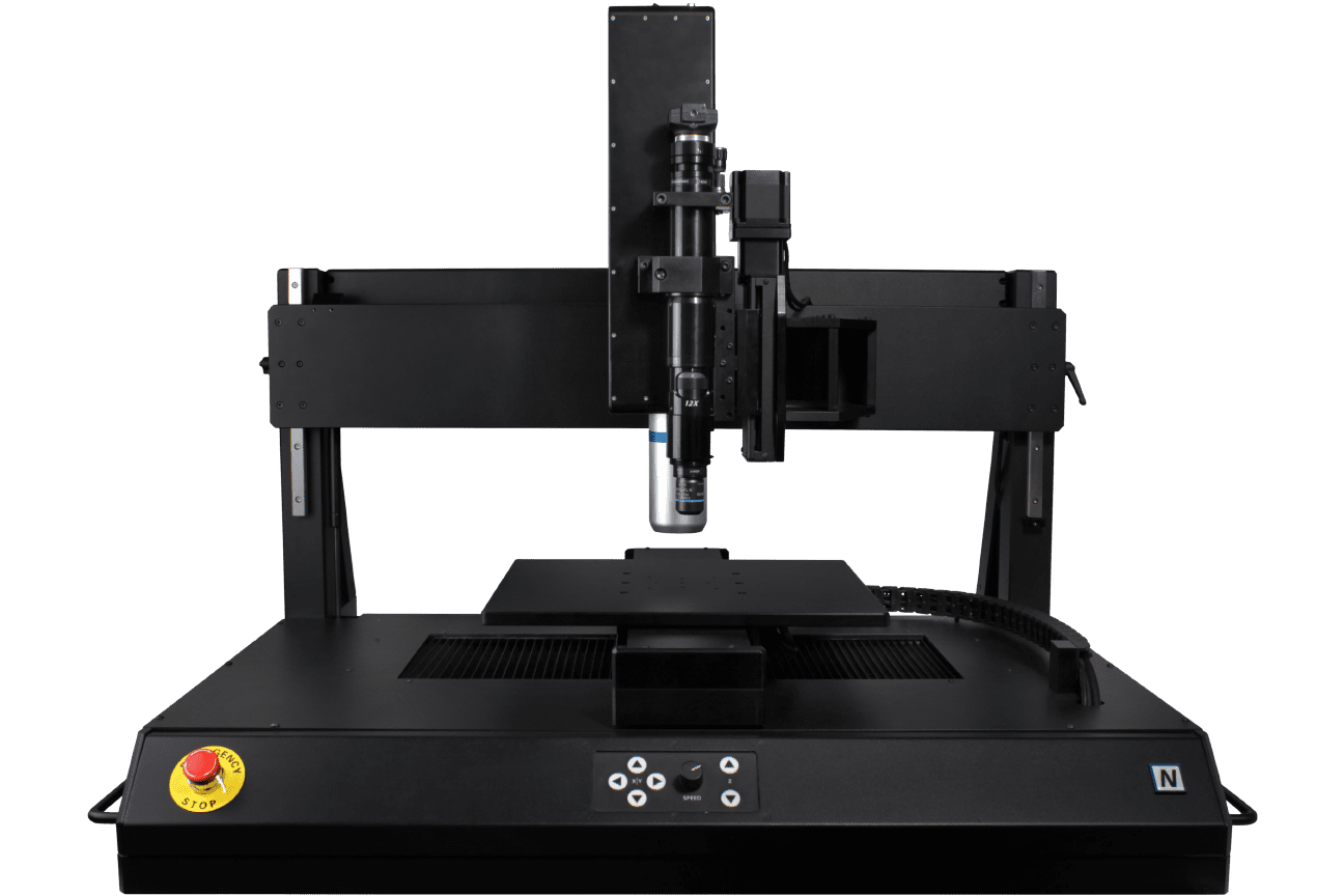
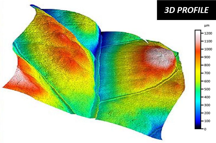
A reliable method is required to quantitatively evaluate the interfacial strength between the polymer coating and the metal substrate. The small diameter of the stent mesh, comparable to a human hair, combined with its three-dimensional geometry, requires:

ultrafine X-Y positioning accuracy
precise control of applied load
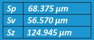
accurate depth measurement during testing

ℹ️ Learn more about nanoindentation and scratch testing lab services for coating adhesion and failure analysis.

Measurement Method

Nano scratch testing is performed using the NANOVEA PB1000 Mechanical Tester, in Nano Scratch Mode, to evaluate the cohesive and adhesive strength of the polymer coating on the metal mesh of stent samples.

Controlled scratch measurements are carried out on stent geometries with dimensions comparable to a human hair, enabling precise evaluation of coating adhesion on complex stent structures.

NANOVEA PB1000 Advanced

Mechanical Tester

Test Conditions

1. Regular Stent Samples

The stent is fixed on the sample stage, with a support wire inserted inside the stent tube to ensure stability during nano scratch testing. The NANOVEA Mechanical Tester is used to perform nano scratch measurements using the parameters summarized in Table 1, to evaluate the cohesive and adhesive strength of the polymer coating on the metal substrate.

Parameter	Value
Load type	Progressive
Initial load	0.05 mN
Final load	300 and 100 mN
Sliding speed	0.5 mm/min
Sliding distance	0.5 mm
Indenter geometry	Conical
Indenter material (tip)	Diamond
Indenter tip radius	20 µm
Temperature	24°C (room)

Table 1: Test parameters for nano scratch measurements on regular stent samples

2. Grooved Stent Samples

The SEM image in Fig. 1 shows the cross-section of the stent sample. The stent features a groove with a depth of approximately 30 µm. The polymer coating, with a thickness of 10.8 µm, is located at the bottom of the groove.

Standard 60° conical diamond tips are not sharp enough to reach the bottom of the groove without contacting the sidewalls. Therefore, a sharper 40° conical diamond tip is used in this study (Fig. 2).

Nano scratch measurements are performed using the parameters summarized in Table 2.

Parameter	Value
Load type	Progressive
Initial load	0.1 mN
Final load	300 mN
Loading rate	300 mN/min
Scratch length	0.25 mm
Scratch speed	0.25 mm/min
Indenter geometry	40° cone
Indenter material (tip)	Diamond
Indenter tip radius	5 µm

Table 2: Test parameters for nano scratch measurements on grooved stent samples

Fig. 1: SEM cross-section of a grooved stent showing polymer coating located at the bottom of the groove, highlighting the challenge of coating adhesion measurement in recessed geometries.

Fig. 2: Schematic of a 40° conical diamond tip designed for nano scratch testing inside stent grooves, enabling accurate adhesion measurement without sidewall interference.

Results and Discussion

The stent mesh has a diameter of approximately 100 μm, comparable to a human hair. Precise positioning is therefore critical to ensure the scratch test is performed at the center of the stent mesh. The NANOVEA Mechanical Tester provides X–Y positioning accuracy down to 0.25 μm, enabling accurate test placement under the integrated optical microscope.

1. Regular Stent Samples

Nano scratch testing is performed with a progressively increasing load up to 300 mN. The full scratch track on the stent is shown in Fig. 3a, while failure behavior at different stages is presented in Fig. 3b and 3c.

Two critical loads are identified:

Lc1: the load at which the first visible damage appears on the coating
Lc2: the load at which the coating is fully removed and the substrate is exposed

The evolution of coefficient of friction (COF) and penetration depth is shown in Fig. 4, providing insight into the progression of coating failure during the test.

The first signs of coating damage appear at Lc1 ≈ 14.5 mN. As the applied load increases, the diamond tip progressively penetrates the polymer coating, resulting in a wider and deeper scratch track. During this phase, the COF increases from approximately 0.05 to 0.7.

At Lc2 ≈ 78.1 mN, the coating is fully delaminated from the metal substrate. Beyond this point, as the load continues to increase, both COF and penetration depth remain relatively stable due to the mechanical support of the underlying metal substrate.

(a) Full Scratch Track

(b) Lc1 ≈ 14.5 mN

Fig. 3: Nano scratch track on a stent coating under progressively increasing load, showing (a) full scratch path, (b) initial coating failure at Lc1 ≈ 14.5 mN, and (c) complete coating delamination at Lc2 ≈ 78.1 mN.

Fig. 4: Evolution of coefficient of friction (COF) and penetration depth during nano scratch testing of a stent coating under progressively increasing load, showing the progression of coating failure and transition to substrate support.

Failures during nano scratch testing up to a maximum load of 300 mN occur at critical loads below 100 mN. To enable a more quantitative comparison of coating performance, additional tests are performed with a maximum load of 100 mN on two stent samples, referred to as Sample 1 and Sample 2.

Fig. 5 compares the scratch tracks of Sample 1 and Sample 2 after nano scratch testing. Sample 1 exhibits the first sign of coating damage at a critical load of Lc1 ≈ 13.2 mN, while Sample 2 shows initial failure at a higher load of Lc1 ≈ 21.1 mN.

Coating delamination occurs at 62.5 mN for Sample 1. In contrast, the coating on Sample 2 remains intact throughout the test, continuing to protect the metal substrate under the same loading conditions.

This behavior is further reflected in the evolution of coefficient of friction (COF) and penetration depth, as shown in Fig. 6. When the diamond tip penetrates through the coating and contacts the metal substrate in Sample 1, the COF reaches a peak while the penetration depth decreases due to the increased stiffness of the underlying substrate.

(a) Sample 1 – Early Coating Failure

(b) Sample 2 – Improved Coating Integrity

Fig. 5: Comparison of nano scratch tracks for two stent coatings, showing (a) early coating failure and delamination in Sample 1, and (b) improved coating integrity in Sample 2 under the same loading conditions.

Fig. 6: Comparison of coefficient of friction (COF) and penetration depth for Sample 1 and Sample 2 during nano scratch testing, showing earlier substrate contact and higher friction response in Sample 1, indicating weaker coating adhesion.

2. Grooved Stent Samples

As shown in Fig. 1 and Fig. 7, the grooved stent mesh has a diameter of approximately 90 μm, comparable to a human hair. The groove has a width of ~50 μm and a depth of 30 μm. This geometry presents a significant challenge for nano scratch testing, particularly for evaluating coating adhesion at the bottom of the groove.

Precise positioning is critical to locate the scratch test within the groove. The nano scratch test is performed with a progressively increasing load up to 300 mN. The full scratch tracks of grooved stent Samples 3 and 4 are compared in Fig. 7.

The critical load Lc is defined as the load at which the coating fails and the substrate becomes exposed. The evolution of normal load and penetration depth, shown in Fig. 8, provides further insight into the progression of coating failure during testing.

As the applied load increases, the diamond tip progressively penetrates the polymer coating, resulting in a deeper scratch track. When the critical load Lc is reached, the coating delaminates from the metal substrate.

Sample 3 exhibits coating failure at Lc ≈ 126 mN, while Sample 4 fails at a higher load of Lc ≈ 173 mN. This difference indicates stronger adhesion of the coating in Sample 4.

The measured critical loads enable quantitative comparison of coating adhesion performance. Under the same testing conditions, the coating on Sample 4 demonstrates higher resistance to delamination, making it the better-performing candidate in this study.

(d) Sample 4 – Higher Adhesion in Groove (Lc ≈ 173 mN)

Fig. 7: Nano scratch tracks inside stent grooves for Samples 3 and 4, showing (c) coating failure at Lc ≈ 126 mN in Sample 3 and (d) higher adhesion with delayed failure at Lc ≈ 173 mN in Sample 4.

(a) Sample 3 – Earlier Coating Failure (Lc ≈ 126 mN)

(b) Sample 4 – Delayed Failure and Higher Adhesion (Lc ≈ 173 mN)

Fig. 8: Evolution of normal load and penetration depth during nano scratch testing inside stent grooves for Samples 3 and 4, showing earlier coating failure in Sample 3 and delayed failure at higher load in Sample 4. The vertical green line indicates the critical load (Lc) where coating delamination occurs.

Conclusion

This study demonstrates the ability of the NANOVEA Mechanical Tester to quantitatively evaluate the cohesive and adhesive strength of polymer coatings on both regular and grooved stent geometries using nano scratch testing.

The recessed geometry of the stent grooves, approximately 50 μm wide and 30 μm deep, presents a significant challenge for coating adhesion measurement. The high X–Y positioning accuracy of 0.25 μm enables precise placement of the scratch test within these confined regions, allowing direct evaluation of coating performance where failure is most critical.

By applying a controlled, progressively increasing load, critical loads associated with coating failure can be identified and compared across samples. This approach enables reliable differentiation of coating adhesion performance and interfacial integrity, even on small, complex stent structures.

References

[I] http://www.nhlbi.nih.gov/health/health-topics/topics/stents
[II] http://www.scielo.org.mx/scielo.php?script=sci_arttext&pid=S1405-99402006000300008

Frequently Asked Questions About Stent Coating Adhesion Testing

What is stent coating adhesion testing?

Stent coating adhesion testing evaluates how strongly a polymer coating is bonded to the metal substrate of a stent. Techniques such as nano scratch testing quantify the load at which coating damage and delamination occur, providing measurable indicators of adhesion strength.

What is critical load (Lc) in nano scratch testing?

Critical load (Lc) is the applied load at which a coating fails during a scratch test.

Lc1 corresponds to the first visible damage in the coating
Lc2 indicates complete coating removal and exposure of the substrate

These values are used to quantify and compare coating adhesion performance.

Why is coating adhesion important in drug-eluting stents?

Coating adhesion directly affects the reliability of drug-eluting stents. Poor adhesion can lead to coating delamination, which may compromise controlled drug release and increase the risk of device failure.

How do you measure coating adhesion inside stent grooves?

Measuring adhesion inside stent grooves requires high positioning accuracy and appropriate indenter geometry. Nano scratch testing with sharp diamond tips allows access to recessed coating regions, enabling direct evaluation of adhesion within complex stent geometries.

What does coefficient of friction (COF) indicate in scratch testing?

The coefficient of friction (COF) reflects changes in surface interaction during the scratch test. A sudden increase in COF often indicates coating failure and contact between the indenter and the underlying metal substrate.

How can nano scratch testing compare different coating formulations?

Nano scratch testing enables direct comparison of coatings by measuring critical loads under controlled conditions. Higher critical loads indicate stronger adhesion and improved resistance to delamination, allowing selection of better-performing coating systems.

Need Reliable Stent Coating Adhesion Testing?

Dental Surface Roughness Measurement & 3D Tooth Topography

Application Note | Dental Surface Characterization

Dental Surface Roughness Measurement and Full 3D Tooth Topography

Surface Roughness Analysis Using Non-Contact Optical Profilometry

Prepared by

Walter Alabiso, PhD; Davide Morrone, MPhys; Andrew Shore, MA

Introduction

The ability to accurately characterize tooth surfaces, including micro-roughness and 3D surface topography at the nanometer scale, enables advanced research and applications in orthodontics and dental materials science. Non-contact optical profilometry provides a precise method for measuring dental surface roughness and analyzing tooth surface morphology without damaging delicate structures. These measurements support the development of composite dental materials that replicate the natural surface roughness of enamel, as well as the design and fabrication of patient-specific dental casts and restorative components.

Low surface roughness plays a primary role in limiting bacterial adhesion and plaque formation, thereby reducing the risk of cavities. An increase in average roughness (Ra) above 2 µm leads to a steep increase in biofilm formation in vivo.¹ An Ra of 0.2 µm is considered the threshold value below which no further reduction in bacterial adhesion can be expected.²

Reconstruction of the tooth’s 3D surface topography enables the fabrication of dental casts, which are essential for accurate diagnosis, treatment planning, and the fabrication of dental appliances.

Non-Contact Optical Profilometry for Dental Surface Analysis

The present study illustrates the potential of NANOVEA’s high-precision non-contact optical profilometers for dental surface roughness measurement and 3D tooth topography analysis. Chromatic Light technology offers significant advantages over classical touch probe techniques. It acquires data points from deep crevices and complex geometries without introducing measurement errors or artifacts caused by local plastic deformation and without requiring extensive data manipulation.

Compared to focus variation systems, single-point optical sensing provides superior lateral and height accuracy, with X/Y resolution below 0.5 µm, maximum vertical resolution of 1.9 nm, and the ability to measure surface angles up to 87°. The technique is effective on transparent, opaque, specular, diffusive, polished, and rough dental surfaces, making it well suited for comprehensive dental surface characterization.

ℹ️ Learn more about non-contact optical profilometry and surface roughness measurement services.

Measurement Method

In this application, the NANOVEA JR25 Non-Contact Optical Profiler was used to analyze the surface roughness and 3D surface topography of an adult human molar previously affected by tooth decay. The side of the tooth was scanned using a PS2–MG140 single-point optical sensor to measure surface roughness parameters over a defined region of interest and along multiple line profiles.

The crown of the tooth was then scanned and reconstructed using a PS5–MG35 single-point optical sensor, which is suited for larger-area acquisition and full 3D tooth topography measurement.

NANOVEA JR25 Portable
Optical Profilometer

Surface Measurement Using NANOVEA Optical Profilometer

Surface roughness measurements were performed on the lateral side of the molar crown, followed by full 3D reconstruction of the crown surface. Separate single-point optical sensors were used to optimize measurement accuracy for both localized roughness analysis and large-area surface topography acquisition.

PS2 – MG140

Surface roughness analysis by area and parallel line profiles on the side of the tooth’s crown.

PS5 – MG35

Full 3D surface reconstruction of the tooth’s crown.

Measurement Parameters

The following measurement parameters were used for localized surface roughness analysis and full 3D surface reconstruction of the molar crown using NANOVEA single-point optical sensors.

Parameter	Roughness Analysis (Area)	Roughness Analysis (Profiles)	Full 3D Reconstruction
Optical Pen	PS2-MG140	PS2-MG140	PS5-MG35
Z-Range [µm]	300	300	10000
X-Distance [mm]	2.00	3.00	7.50
X-Step Size [µm]	1.70	1.70	10.00
Y-Distance [mm]	2.00	1.00	7.00
Y-Step Size [µm]	1.70	100.00	10.00
Average (Avg)	1	1	1
Measurement Type	Direct	Direct	Direct
Acquisition Mode	Single Frequency	Single Frequency	Double Frequency
Acquisition Rate [Hz]	200	200	100–400
Light Intensity [%]	100	100	100

Optical Profilometry Results

Surface Roughness Analysis (Area)

The PS2 single-point optical sensor was used to investigate fine surface features on the side of the tooth. The image below shows a false-color 2D surface map of the scanned region obtained by non-contact optical profilometry.

A least-squares degree-8 polynomial form removal was applied to isolate the surface roughness component. The roughness filters S-Gaussian 2.5 µm and L-Gaussian 0.8 mm were then applied according to ISO 25178. The resulting filtered surface and corresponding roughness parameters are presented below.

ISO 25178 – Roughness (S-L)
S-filter (λs): Gaussian, 2.5 µm
F: [Workflow] Form removed (LS-poly 8)
L-filter (λc): Gaussian, 0.8 mm
Height Parameters
Sq	2.433	µm	Root-mean-square height
Ssk	-0.102		Skewness
Sku	3.715		Kurtosis
Sp	18.861	µm	Maximum peak height
Sv	16.553	µm	Maximum pit depth
Sz	35.414	µm	Maximum height
Sa	1.888	µm	Arithmetic mean height

The average surface roughness Sa is 1.888 µm, while the peak-to-valley height Sz reaches 35.414 µm.

A 3D surface rendering of the filtered area is shown below for visualization.

Roughness Analysis (Profiles)

Surface roughness profiles were measured using a series of 11 parallel line scans along the X direction on the side of the tooth. The false-color 2D surface map of the raw scan is shown below.

The surface form was removed using a least-squares 8-degree polynomial prior to applying the metrological filters, leaving the residual surface shown below.

A statistical analysis of the measured surface roughness profiles reveals the following line roughness parameters.

		Description	Mean	Std dev	Min	Max
ISO 4287 – Roughness (S-L)
F: None
S-filter (λs): Gaussian, 2.5 µm
L-filter (λc): Gaussian, 0.8 mm
Evaluation length: All λc (3)
Amplitude Parameters – Roughness Profile
Rp	µm	Maximum peak height of the roughness profile	5.683	0.761	4.315	6.610
Rv	µm	Maximum valley depth of the roughness profile	6.242	1.009	4.701	8.438
Rz	µm	Maximum height of roughness profile	11.925	1.676	9.123	15.048
Ra	µm	Arithmetic mean deviation of the roughness profile	2.063	0.297	1.710	2.629
Rq	µm	Root-mean-square (RMS) deviation of the roughness profile	2.523	0.361	2.057	3.175

F: None

S-filter (λs): Gaussian, 2.5 µm

L-filter (λc): Gaussian, 0.8 mm

Evaluation length: All λc (3)

The value of Ra is consistent with the Sa value extracted from the surface area measurement.

Different metrological filters can be applied to distinguish between macroscopic waviness and microscopic surface roughness. For example, a coarser filter cut-off, such as the 8 mm cut-off used with the Robust Gaussian order-2 filter, produces a smoother waviness profile (red) that is less sensitive to sharp local variations and follows the original surface profile more loosely.

Alternatively, a finer cut-off (e.g., 0.08 mm) enables the analysis of micro-roughness by removing the waviness component that follows the original profile at a larger scale, leaving the finer surface roughness features of the tooth visible.

The microroughness analysis obtained using a 0.08 mm L-Gaussian filter is presented below.

		Description	Mean	Std dev	Min	Max
ISO 4287 – Roughness (S-L)
F: None
S-filter (λs): Gaussian, 2.5 µm
L-filter (λc): Gaussian, 0.08 mm
Evaluation length: All λc (37)
Amplitude Parameters – Roughness Profile
Rp	µm	Maximum peak height of the roughness profile	1.582	0.122	1.342	1.748
Rv	µm	Maximum valley depth of the roughness profile	1.466	0.119	1.254	1.661
Rz	µm	Maximum height of roughness profile	3.049	0.196	2.820	3.409
Ra	µm	Arithmetic mean deviation of the roughness profile	0.495	0.047	0.423	0.597
Rq	µm	Root-mean-square (RMS) deviation of the roughness profile	0.643	0.056	0.562	0.762

F: None

S-filter (λs): Gaussian, 2.5 µm

L-filter (λc): Gaussian, 0.8 mm

Evaluation length: All λc (3)

Full 3D Tooth Surface Topography Reconstruction

The extended Z-scan range of the PS5 optical sensor enables high-fidelity scanning of the entire tooth crown surface. The resulting 3D surface topography is shown below.

2D VIEW: 2D surface map of the tooth crown measured with optical profilometry

3D VIEW: High-fidelity 3D rendering of the molar crown surface obtained with optical profilometry

Conclusion

In this application, the NANOVEA JR25 Non-Contact Optical Profiler was used to measure the surface roughness and 3D surface topography of an adult human molar.

Both the area scan and the line profile analysis revealed a roughness Rq of approximately 2.5 µm and an Ra of about 1.9–2.0 µm. These values are consistent with results reported in the literature.³ The use of a narrower L-Gaussian filter with an 80 µm cut-off enabled further investigation of micro-roughness, revealing an Rq of 0.643 µm and an Ra of 0.495 µm.

The full 3D surface topography of the molar crown was reconstructed with high fidelity. The high measurement resolution allows detection of fine surface features and crevices. The resulting surface data can be easily processed and exported as STL files, enabling the design and fabrication of customized dental devices and restorative components.

References

[1] Shin, B.W., et al. Surface Roughness of Prefabricated Pediatric Zirconia Crowns Following Simulated Toothbrushing. Pediatric Dentistry 44.5 (2022): 363–367.
[2] Bollen, C.M.L., Paul Lambrechts, and Marc Quirynen. Comparison of surface roughness of oral hard materials to the threshold surface roughness for bacterial plaque retention: A review of the literature. Dental Materials 13.4 (1997): 258–269.
[3] Suputtamongkol, K., et al. Surface roughness resulting from wear of lithia-disilicate-based posterior crowns. Wear 269.3–4 (2010): 317–322.

Frequently Asked Questions About Dental Surface Roughness Measurement

What is dental surface roughness measurement?

Dental surface roughness measurement quantifies the microscopic texture of tooth surfaces using parameters such as Ra, Rq, and Sa. Optical profilometers measure these features without contacting the surface, allowing accurate analysis of enamel, restorative materials, and dental crowns.

Why use optical profilometry to measure tooth roughness?

Optical profilometry provides non-contact surface measurement with nanometer-scale vertical resolution. It captures 2D surface maps and full 3D surface topography of dental structures without damaging soft or polished surfaces.

What roughness parameters are used for dental surface analysis?

Common roughness parameters include Ra (arithmetic mean roughness), Rq (root mean square roughness), Sa (areal roughness), and Sz (maximum surface height). These parameters help evaluate enamel wear, plaque adhesion risk, and the performance of restorative materials.

Why is surface roughness important in dentistry?

Surface roughness affects plaque retention, wear resistance, and the long-term performance of dental restorations. Controlling micro-roughness can reduce bacterial adhesion and improve the durability of dental materials.

Need Reliable Surface Roughness Measurement for Dental Materials?

Shot Peened Surface Analysis

SHOT PEENED SURFACE ANALYSIS

USING 3D NON-CONTACT PROFILOMETER

Prepared by

CRAIG LEISING

INTRODUCTION

Shot peening is a process in which a substrate is bombarded with spherical metal, glass, or ceramic beads—commonly referred to as “shot”—at a force intended to induce plasticity on the surface. Analyzing the characteristics before and after peening provides crucial insights for enhancing process comprehension and control. The surface roughness and coverage area of dimples left by the shot are especially noteworthy aspects of interest.

Importance of 3D Non-Contact Profilometer for Shot-Peened Surface Analysis

Unlike traditional contact profilometers, which have traditionally been used for shot-peened surface analysis, 3D non-contact measurement provides a complete 3D image to offer a more comprehensive understanding of coverage area and surface topography. Without 3D capabilities, an inspection will solely rely on 2D information, which is insufficient for characterizing a surface. Understanding the topography, coverage area, and roughness in 3D is the best approach for controlling or improving the peening process. NANOVEA’s 3D Non-Contact Profilometers utilize Chromatic Light technology with a unique capability to measure steep angles found on machined and peened surfaces. Additionally, when other techniques fail to provide reliable data due to probe contact, surface variation, angle, or reflectivity, NANOVEA Profilometers succeed.

MEASUREMENT OBJECTIVE

In this application, the NANOVEA ST400 Non-Contact Profilometer is used to measure raw material and two differently peened surfaces for a comparative review. There is an endless list of surface parameters that can be automatically calculated after the 3D surface scan. Here, we will review the 3D surface and select areas of interest for further analysis, including quantifying and investigating the roughness, dimples, and surface area.

NANOVEA ST400 Standard
Optical 3D Profilometer

THE SAMPLE

RESULTS

STEEL SURFACE

ISO 25178 3D ROUGNESS PARAMETERS

SA	0.399 μm	Average Roughness
Sq	0.516 μm	RMS Roughness
Sz	5.686 μm	Maximum Peak-to-Valley
Sp	2.976 μm	Maximum Peak Height
Sv	2.711 μm	Maximum Pit Depth
Sku	3.9344	Kurtosis
Ssk	-0.0113	Skewness
Sal	0.0028 mm	Auto-Correlation Length
Str	0.0613	Texture Aspect Ratio
Sdar	26.539 mm²	Surface Area
Svk	0.589 μm	Reduced Valley Depth

RESULTS

PEENED SURFACE 1

SURFACE COVERAGE 98.105%

ISO 25178 3D ROUGNESS PARAMETERS

Sa	4.102 μm	Average Roughness
Sq	5.153 μm	RMS Roughness
Sz	44.975 μm	Maximum Peak-to-Valley
Sp	24.332 μm	Maximum Peak Height
Sv	20.644 μm	Maximum Pit Depth
Sku	3.0187	Kurtosis
Ssk	0.0625	Skewness
Sal	0.0976 mm	Auto-Correlation Length
Str	0.9278	Texture Aspect Ratio
Sdar	29.451 mm²	Surface Area
Svk	5.008 μm	Reduced Valley Depth

RESULTS

PEENED SURFACE 2

SURFACE COVERAGE 97.366%

ISO 25178 3D ROUGNESS PARAMETERS

Sa	4.330 μm	Average Roughness
Sq	5.455 μm	RMS Roughness
Sz	54.013 μm	Maximum Peak-to-Valley
Sp	25.908 μm	Maximum Peak Height
Sv	28.105 μm	Maximum Pit Depth
Sku	3.0642	Kurtosis
Ssk	0.1108	Skewness
Sal	0.1034 mm	Auto-Correlation Length
Str	0.9733	Texture Aspect Ratio
Sdar	29.623 mm²	Surface Area
Svk	5.167 μm	Reduced Valley Depth

CONCLUSION

In this shot-peened surface analysis application, we have demonstrated how the NANOVEA ST400 3D Non-Contact Profiler precisely characterizes both the topography and nanometer details of a peened surface. It is evident that both Surface 1 and Surface 2 have a significant impact on all the parameters reported here when compared to the raw material. A simple visual examination of the images reveals the differences between the surfaces. This is further confirmed by observing the coverage area and the listed parameters. In comparison to Surface 2, Surface 1 exhibits a lower average roughness (Sa), shallower dents (Sv), and reduced surface area (Sdar), but a slightly higher coverage area.

From these 3D surface measurements, areas of interest can be readily identified and subjected to a comprehensive array of measurements, including Roughness, Finish, Texture, Shape, Topography, Flatness, Warpage, Planarity, Volume, Step-Height, and others. A 2D cross-section can quickly be chosen for detailed analysis. This information allows for a comprehensive investigation of peened surfaces, utilizing a complete range of surface measurement resources. Specific areas of interest could be further examined with an integrated AFM module. NANOVEA 3D Profilometers offer speeds of up to 200 mm/s. They can be customized in terms of size, speeds, scanning capabilities, and can even comply with Class 1 Clean Room standards. Options like Indexing Conveyor and integration for Inline or Online usage are also available.

A special thanks to Mr. Hayden at IMF for supplying the sample shown in this note. Industrial Metal Finishing Inc. | indmetfin.com

Got a similar application?

Paint Surface Morphology

PAINT SURFACE MORPHOLOGY

AUTOMATED REAL-TIME EVOLUTION MONITORING
USING NANOVEA 3D PROFILOMETER

Prepared by

DUANJIE LI, PhD

INTRODUCTION

Protective and decorative properties of paint play a significant role in a variety of industries, including automotive, marine, military, and construction. To achieve desired properties, such as corrosion resistance, UV protection, and abrasion resistance, paint formulas and architectures are carefully analyzed, modified, and optimized.

IMPORTANCE OF 3D NON-CONTACT PROFILOMETER FOR DRYING PAINT SURFACE MORPHOLOGY ANALYSIS

Paint is usually applied in liquid form and undergoes a drying process, which involves the evaporation of solvents and the transformation of the liquid paint into a solid film. During the drying process, the paint surface progressively changes its shape and texture. Different surface finishes and textures can be developed by using additives to modify the surface tension and flow properties of the paint. However, in cases of a poorly formulated paint recipe or improper surface treatment, undesired paint surface failures may occur.

Accurate in situ monitoring of the paint surface morphology during the drying period can provide direct insight into the drying mechanism. Moreover, real-time evolution of surface morphologies is very useful information in various applications, such as 3D printing. The NANOVEA 3D Non-Contact Profilometers measure the paint surface morphology of materials without touching the sample, avoiding any shape alteration that may be caused by contact technologies such as a sliding stylus.

MEASUREMENT OBJECTIVE

In this application, the NANOVEA ST500 Non-Contact Profilometer, equipped with a high-speed line optical sensor, is used to monitor the paint surface morphology during its 1-hour drying period. We showcase the NANOVEA Non-Contact Profilometer’s capability in providing automated real-time 3D profile measurement of materials with continuous shape change.

NANOVEA ST500 Large Area
Optical 3D Profilometer

RESULTS & DISCUSSION

The paint was applied on the surface of a metal sheet, followed immediately by automated measurements of the morphology evolution of the drying paint in situ using the NANOVEA ST500 Non-Contact Profilometer equipped with a high-speed line sensor. A macro had been programmed to automatically measure and record the 3D surface morphology at specific time intervals: 0, 5, 10, 20, 30, 40, 50, and 60 min. This automated scanning procedure enables users to perform scanning tasks automatically by running set procedures in sequence, significantly reducing effort, time, and possible user errors compared to manual testing or repeated scans. This automation proves to be extremely useful for long-term measurements involving multiple scans at different time intervals.

The optical line sensor generates a bright line consisting of 192 points, as shown in FIGURE 1. These 192 light points scan the sample surface simultaneously, significantly increasing the scanning speed. This ensures that each 3D scan is completed quickly to avoid substantial surface changes during each individual scan.

FIGURE 1: Optical line sensor scanning the surface of the drying paint.

The false color view, 3D view, and 2D profile of the drying paint topography at representative times are shown in FIGURE 2, FIGURE 3, and FIGURE 4, respectively. The false color in the images facilitates the detection of features that are not readily discernible. Different colors represent height variations across different areas of the sample surface. The 3D view provides an ideal tool for users to observe the paint surface from different angles. During the first 30 minutes of the test, the false colors on the paint surface gradually change from warmer tones to cooler ones, indicating a progressive decrease in height over time in this period. This process slows down, as shown by the mild color change when comparing the paint at 30 and 60 minutes.

The average sample height and roughness Sa values as a function of the paint drying time are plotted in FIGURE 5. The full roughness analysis of the paint after 0, 30, and 60 min drying time are listed in TABLE 1. It can be observed that the average height of the paint surface rapidly decreases from 471 to 329 µm in the first 30 min of drying time. The surface texture develops at the same time as the solvent vaporizes, leading to an increased roughness Sa value from 7.19 to 22.6 µm. The paint drying process slows down thereafter, resulting in a gradual decrease of the sample height and Sa value to 317 µm and 19.6 µm, respectively, at 60 min.

This study highlights the capabilities of the NANOVEA 3D Non-Contact Profilometer in monitoring the 3D surface changes of the drying paint in real-time, providing valuable insights into the paint drying process. By measuring the surface morphology without touching the sample, the profilometer avoids introducing shape alterations to the undried paint, which can occur with contact technologies like sliding stylus. This non-contact approach ensures accurate and reliable analysis of drying paint surface morphology.

FIGURE 2: Evolution of the drying paint surface morphology at different times.

FIGURE 3: 3D view of the paint surface evolution at different drying times.

FIGURE 4: 2D profile across the paint sample after different drying times.

FIGURE 5: Evolution of the average sample height and roughness value Sa as a function of the paint drying time.

ISO 25178 - Surface Texture Parameters

Drying time (min)	0	5	10	20	30	40	50	60
Sq (µm)	7.91	9.4	10.8	20.9	22.6	20.6	19.9	19.6
Sku	26.3	19.8	14.6	11.9	10.5	9.87	9.83	9.82
Sp (µm)	97.4	105	108	116	125	118	114	112
Sv (µm)	127	70.2	116	164	168	138	130	128
Sz (µm)	224	175	224	280	294	256	244	241
Sa (µm)	4.4	5.44	6.42	12.2	13.3	12.2	11.9	11.8

TABLE 1: Paint roughness at different drying times.

CONCLUSION

In this application, we have showcased the capabilities of the NANOVEA ST500 3D Non-Contact Profilometer in monitoring the evolution of paint surface morphology during the drying process. The high-speed optical line sensor, generating a line with 192 light spots that scan the sample surface simultaneously, has made the study time-efficient while ensuring unmatched accuracy.

The macro function of the acquisition software allows for programming automated measurements of the 3D surface morphology in situ, making it particularly useful for long-term measurement involving multiple scans at specific target time intervals. It significantly reduces the time, effort, and potential for user errors. The progressive changes in surface morphology are continuously monitored and recorded in real-time as the paint dries, providing valuable insights into the paint drying mechanism.

The data shown here represents only a fraction of the calculations available in the analysis software. NANOVEA Profilometers are capable of measuring virtually any surface, whether it’s transparent, dark, reflective, or opaque.

Got a similar application?

Fractography Analysis Using 3D Profilometry

FRACTOGRAPHY ANALYSIS

USING 3D PROFILOMETRY

Prepared by

CRAIG LEISING

INTRODUCTION

Fractography is the study of features on fractured surfaces and has historically been investigated via Microscope or SEM. Depending on the size of the feature, a microscope (macro features) or SEM (nano and micro features) are selected for the surface analysis. Both ultimately allowing for the identification of the fracture mechanism type. Although effective, the Microscope has clear limitations and the SEM in most cases, other than atomic-level analysis, is unpractical for fracture surface measurement and lacks broader use capability. With advances in optical measurement technology, the NANOVEA 3D Non-Contact Profilometer is now considered the instrument of choice, with its ability to provide nano through macro-scale 2D & 3D surface measurements

IMPORTANCE OF 3D NON-CONTACT PROFILOMETER FOR FRACTURE INSPECTION

Unlike an SEM, a 3D Non-Contact Profilometer can measure nearly any surface, sample size, with minimal sample prep, all while offering superior vertical/horizontal dimensions to that of an SEM. With a profiler, nano through macro range features are captured in a single measurement with zero influence from sample reflectivity. Easily measure any material: transparent, opaque, specular, diffusive, polished, rough etc. The 3D Non-Contact Profilometer provides broad and user-friendly capability to maximize surface fracture studies at a fraction of the cost of an SEM.

MEASUREMENT OBJECTIVE

In this application, the NANOVEA ST400 is used to measure the fractured surface of a steel sample. In this study, we will showcase a 3D area, 2D profile extraction and surface directional map of the surface.

NANOVEA

ST400

RESULTS

TOP SURFACE

3D Surface Texture Direction

Isotropy	51.26%
First Direction	123.2º
Second Direction	116.3º
Third Direction	0.1725º

Surface Area, Volume, Roughness and many others can be automatically calculated from this extraction.

2D Profile Extraction

RESULTS

SIDE SURFACE

3D Surface Texture Direction

Isotropy	15.55%
First Direction	0.1617º
Second Direction	110.5º
Third Direction	171.5º

Surface Area, Volume, Roughness and many others can be automatically calculated from this extraction.

2D Profile Extraction

CONCLUSION

In this application, we have shown how the NANOVEA ST400 3D Non-Contact Profilometer can precisely characterize the full topography (nano, micro and macro features) of a fractured surface. From the 3D area, the surface can be clearly identified and subareas or profiles/cross-sections can be quickly extracted and analyzed with an endless list of surface calculations. Sub nanometer surface features can be further analyzed with an integrated AFM module.

Additionally, NANOVEA has included a portable version to their Profilometer line-up, especially critical for field studies where a fracture surface is immovable. With this broad list of surface measurement capabilities, fracture surface analysis has never been easier and more convenient with a single instrument.

Got a similar application?

Fiberglass Surface Topography Using 3D Profilometry

FIBERGLASS SURFACE TOPOGRAPHY

USING 3D PROFILOMETRY

Prepared by

CRAIG LEISING

INTRODUCTION

Fiberglass is a material made from extremely fine fibers of glass. It is used as a reinforcing agent for many polymer products; the resulting composite material, properly known as fiber-reinforced polymer (FRP) or glass-reinforced plastic (GRP), is called “fiberglass” in popular usage.

IMPORTANCE OF SURFACE METROLOGY INSPECTION FOR QUALITY CONTROL

Although there are many uses for Fiberglass reinforcement, in most applications it is crucial that they are as strong as possible. Fiberglass composites have one of the highest strength to weight ratios available and in some cases, pound for pound it is stronger than steel. Aside from high strength, it is also important to have the smallest possible exposed surface area. Large fiberglass surfaces can make the structure more vulnerable to chemical attack and possibly material expansion. Therefore, surface inspection is critical to quality control production.

MEASUREMENT OBJECTIVE

In this application, the NANOVEA ST400 is used to measure a Fiberglass Composite surface for roughness and flatness. By quantifying these surface features it is possible to create or optimize a stronger, longer lasting fiberglass composite material.

NANOVEA

ST400

MEASUREMENT PARAMETERS

PROBE	1 mm
ACQUISITION RATE	300 Hz
AVERAGING	1
MEASURED SURFACE	5 mm x 2 mm
STEP SIZE	5 µm x 5 µm
SCANNING MODE	Constant speed

PROBE SPECIFICATIONS

**MEASUREMENT RANGE**	1 mm
Z RESOLUTION	25 nm
Z ACCURACY	200 nm
LATERAL RESOLUTION	2 μm

RESULTS

FALSE COLOR VIEW

3D Surface Flatness

3D Surface Roughness

Sa	15.716 μm	Arithmetical Mean Height
Sq	19.905 μm	Root Mean Square Height
Sp	116.74 μm	Maximum Peak Height
Sv	136.09 μm	Maximum Pit Height
Sz	252.83 μm	Maximum Height
Ssk	0.556	Skewness
Ssu	3.654	Kurtosis

CONCLUSION

As shown in the results, the NANOVEA ST400 Optical Profiler was able to accurately measure the roughness and flatness of the fiberglass composite surface. Data can be measured over multiple batches of fiber composites and or a given time period to provide crucial information about different fiberglass manufacturing processes and how they react over time. Thus, the ST400 is a viable option for strengthening the quality control process of fiberglass composite materials.

Got a similar application?

Polymer Belt Wear and Friction using a Tribometer

POLYMER BELTS

WEAR AND FRICTION USING a TRIBOMETER

Prepared by

DUANJIE LI, PhD

INTRODUCTION

Belt drive transmits power and tracks relative movement between two or more rotating shafts. As a simple and inexpensive solution with minimal maintenance, belt drives are widely used in a variety of applications, such as bucksaws, sawmills, threshers, silo blowers and conveyors. Belt drives can protect the machinery from overload as well as damp and isolate vibration.

IMPORTANCE OF WEAR EVALUATION FOR BELT DRIVES

Friction and wear are inevitable for the belts in a belt-driven machine. Sufficient friction ensures effective power transmission without slipping, but excessive friction may rapidly wear the belt. Different types of wear such as fatigue, abrasion and friction take place during the belt drive operation. In order to extend the lifetime of the belt and to cut the cost and time on belt repairing and replacement, reliable evaluation of the wear performance of the belts is desirable in improving belt lifespan, production efficiency and application performance. Accurate measurement of the coefficient of friction and wear rate of the belt facilitates R&D and quality control of belt production.

MEASUREMENT OBJECTIVE

In this study, we simulated and compared the wear behaviors of belts with different surface textures to showcase the capacity of the NANOVEA T2000 Tribometer in simulating the wear process of the belt in a controlled and monitored manner.

NANOVEA

T2000

TEST PROCEDURES

The coefficient of friction, COF, and the wear resistance of two belts with different surface roughness and texture were evaluated by the NANOVEA High-Load Tribometer using Linear Reciprocating Wear Module. A Steel 440 ball (10 mm diameter) was used as the counter material. The surface roughness and wear track were examined using an integrated 3D Non-Contact profilometer. The wear rate, K, was evaluated using the formula K=Vl(Fxs), where V is the worn volume, F is the normal load and s is the sliding distance.

Please note that a smooth Steel 440 ball counterpart was used as an example in this study, any solid material with different shapes and surface finish can be applied using custom fixtures to simulate the actual application situation.

RESULTS & DISCUSSION

The Textured Belt and Smooth Belt have a surface roughness Ra of 33.5 and 8.7 um, respectively, according to the analyzed surface profiles taken with a NANOVEA 3D Non-Contact Optical profiler. The COF and wear rate of the two tested belts were measured at 10 N and 100 N, respectively, to compare the wear behavior of the belts at different loads.

FIGURE 1 shows the evolution of COF of the belts during the wear tests. The belts with different textures exhibit substantially different wear behaviors. It is interesting that after the run-in period during which the COF progressively increases, the Textured Belt reaches a lower COF of ~0.5 in both the tests conducted using loads of 10 N and 100 N. In comparison, the Smooth Belt tested under the load of 10 N exhibits a significantly higher COF of~ 1.4 when the COF gets stable and maintains above this value for the rest of the test. The Smooth Belt tested under the load of 100 N rapidly was worn out by the steel 440 ball and formed a large wear track. The test was therefore stopped at 220 revolutions.

FIGURE 1: Evolution of COF of the belts at different loads.

FIGURE 2 compares the 3D wear track images after the tests at 100 N. The NANOVEA 3D non-contact profilometer offers a tool to analyze the detailed morphology of the wear tracks, providing more insight in fundamental understanding of wear mechanism.

TABLE 1: Result of wear track analysis.

FIGURE 2: 3D view of the two belts
after the tests at 100 N.

The 3D wear track profile allows direct and accurate determination of the wear track volume calculated by the advanced analysis software as shown in TABLE 1. In a wear test for 220 revolutions, the Smooth Belt has a much larger and deeper wear track with a volume of 75.7 mm3, compared to a wear volume of 14.0 mm3 for the Textured Belt after a 600-revolution wear test. The significantly higher friction of the Smooth Belt against the steel ball leads to a 15 fold higher wear rate compared to the Textured Belt.

Such a drastic difference of COF between the Textured Belt and Smooth Belt is possibly related to the size of the contact area between the belt and the steel ball, which also leads to their different wear performance. FIGURE 3 shows the wear tracks of the two belts under the optical microscope. The wear track examination is in agreement with the observation on COF evolution: The Textured Belt, which maintains a low COF of ~0.5, exhibits no sign of wear after the wear test under a load of 10 N. The Smooth Belt shows a small wear track at 10 N. The wear tests carried out at 100 N create substantially larger wear tracks on both the Textured and Smooth Belts, and the wear rate will be calculated using 3D profiles as will be discussed in the following paragraph.

FIGURE 3: Wear tracks under optical microscope.

CONCLUSION

In this study, we showcased the capacity of the NANOVEA T2000 Tribometer in evaluating the coefficient of friction and wear rate of belts in a well-controlled and quantitative manner. The surface texture plays a critical role in the friction and wear resistance of the belts during their service performance. The textured belt exhibits a stable coefficient of friction of ~0.5 and possesses a long lifetime, which results in reduced time and cost on tool repairing or replacement. In comparison, the excessive friction of the smooth belt against the steel ball rapidly wears the belt. Further, the loading on the belt is a vital factor of its service lifetime. Overload creates very high friction, leading to accelerated wear to the belt.

The NANOVEA T2000 Tribometer offers precise and repeatable wear and friction testing using ISO and ASTM compliant rotative and linear modes, with optional high temperature wear, lubrication and tribocorrosion modules available in one pre-integrated system. NANOVEA’s unmatched range is an ideal solution for determining the full range of tribological properties of thin or thick, soft or hard coatings, films and substrates.

Got a similar application?

Fossil Microstructure Using 3D Profilometry

FOSSIL MICROSTRUCTURE

USING 3D PROFILOMETRY

Prepared by

DUANJIE LI, PhD

INTRODUCTION

Fossils are the preserved remains of traces of plants, animals and other organisms buried in sediment under ancient seas, lakes and rivers. The soft body tissue usually decays after death, but the hard shells, bones and teeth fossilize. Microstructure surface features are often preserved when mineral replacement of the original shells and bones takes place, which provides an insight into the evolution of weather and the formation mechanism of fossils.

IMPORTANCE OF A 3D NON-CONTACT PROFILOMETER FOR FOSSIL EXAMINATION

3D profiles of the fossil enable us to observe the detailed surface features of the fossil sample from a closer angle. The high resolution and accuracy of the NANOVEA profilometer may not be discernible by the naked eye. The profilometer’s analysis software offers a wide range of studies applicable to these unique surfaces. Unlike other techniques such as touch probes, the NANOVEA 3D Non-Contact Profilometer measures the surface features without touching the sample. This allows for the preservation of the true surface features of certain delicate fossil samples. Moreover, the portable model Jr25 profilometer enables 3D measurement on fossil sites, which substantially facilitates fossil analysis and protection after excavation.

MEASUREMENT OBJECTIVE

In this study, the NANOVEA Jr25 Profilometer is used to measure the surface of two representative fossil samples. The entire surface of each fossil was scanned and analyzed in order to characterize its surface features which include roughness, contour and texture direction.

NANOVEA

Jr25

BRACHIOPOD FOSSIL

The first fossil sample presented in this report is a Brachiopod fossil, which came from a marine animal that has hard “valves” (shells) on its upper and lower surfaces. They first appeared in the Cambrian period, which is more than 550 million years ago.

The 3D View of the scan is shown in FIGURE 1 and False Color View is shown in FIGURE 2.

FIGURE 1: 3D View of the Brachiopod fossil sample.

FIGURE 2: False Color View of the Brachiopod fossil sample.

The overall form was then removed from the surface in order to investigate the local surface morphology and contour of the Brachiopod fossil as shown in FIGURE 3. A peculiar divergent groove texture can now be observed on the Brachiopod fossil sample.

FIGURE 3: False Color View and Contour Lines View after form removal.

A line profile is extracted from the textured area to show a crossectional view of the fossil surface in FIGURE 4. The Step Height study measures precise dimensions of the surface features. The grooves possess an average width of ~0.38 mm and depth of ~0.25 mm.

FIGURE 4: Line profile and Step Height studies of the textured surface.

CRINOID STEM FOSSIL

The second fossil sample is a Crinoid stem fossil. Crinoids first appeared in the seas of the Middle Cambrian Period, about 300 million years before dinosaurs.

The 3D View of the scan is shown in FIGURE 5 and False Color View is shown in FIGURE 6.

FIGURE 5: 3D View of the Crinoid fossil sample.

The surface texture isotropy and roughness of the Crinoid stem fossil are analyzed in FIGURE 7.

This fossil has a preferential texture direction in the angle close to 90°, leading to texture isotropy of 69%.

FIGURE 6: False Color View of the Crinoid stem sample.

FIGURE 7: Surface texture isotropy and roughness of the Crinoid stem fossil.

The 2D profile along the axial direction of the Crinoid stem fossil is shown in FIGURE 8.

The size of the peaks of the surface texture is fairly uniform.

FIGURE 8: 2D profile analysis of the Crinoid stem fossil.

CONCLUSION

In this application, we comprehensively studied the 3D surface features of a Brachiopod and Crinoid stem fossil using the NANOVEA Jr25 Portable Non-Contact Profilometer. We showcase that the instrument can precisely characterize the 3D morphology of the fossil samples. The interesting surface features and texture of the samples are then further analyzed. The Brachiopod sample possesses a divergent groove texture, while the Crinoid stem fossil shows preferential texture isotropy. The detailed and precise 3D surface scans prove to be ideal tools for palaeontologists and geologists to study the evolution of lives and the formation of fossils.

The data shown here represent only a portion of the calculations available in the analysis software. NANOVEA Profilometers measure virtually any surface in fields including Semiconductor, Microelectronics, Solar, Fiber Optics, Automotive, Aerospace, Metallurgy, Machining, Coatings, Pharmaceutical, Biomedical, Environmental and many others.

Got a similar application?

Processed Leather Surface Finish using 3D Profilometry

PROCESSED LEATHER

SURFACE FINISH USING 3D PROFILOMETRY

Prepared by

CRAIG LEISING

INTRODUCTION

Once the tanning process of a leather hide is complete the leather surface can undergo several finishing processes for a variety of looks and touch. These mechanical processes can include stretching, buffing, sanding, embossing, coating etc. Dependent upon the end use of the leather some may require a more precise, controlled and repeatable processing.

IMPORTANCE OF PROFILOMETRY INSPECTION FOR R&D AND QUALITY CONTROL

Due to the large variation and unreliability of visual inspection methods, tools that are capable of accurately quantifying micro and nano scales features can improve leather finishing processes. Understanding the surface finish of leather in a quantifiable sense can lead to improved data driven surface processing selection to achieve optimal finish results. NANOVEA 3D Non-Contact Profilometers utilize chromatic confocal technology to measure finished leather surfaces and offer the highest repeatability and accuracy in the market. Where other techniques fail to provide reliable data, due to probe contact, surface variation, angle, absorption or reflectivity, NANOVEA Profilometers succeed.

MEASUREMENT OBJECTIVE

In this application, the NANOVEA ST400 is used to measure and compare the surface finish of two different but closely processed leather samples. Several surface parameters are automatically calculated from the surface profile.

Here we will focus on surface roughness, dimple depth, dimple pitch and dimple diameter for comparative evaluation.

NANOVEA

ST400

RESULTS: SAMPLE 1

ISO 25178

HEIGHT PARAMETERS

OTHER 3D PARAMETERS

RESULTS: SAMPLE 2

ISO 25178

HEIGHT PARAMETERS

OTHER 3D PARAMETERS

DEPTH COMPARATIVE

Depth distribution for each sample.
A large number of deep dimples were observed in SAMPLE 1.

PITCH COMPARATIVE

Pitch between dimples on SAMPLE 1 is slightly smaller
than SAMPLE 2, but both have a similar distribution

MEAN DIAMETER COMPARATIVE

Similar distributions of mean diameter of dimples,
with SAMPLE 1 showing slightly smaller mean diameters on average.

CONCLUSION

In this application, we have shown how the NANOVEA ST400 3D Profilometer can precisely characterize the surface finish of processed leather. In this study, having the ability to measure surface roughness, dimple depth, dimple pitch and dimple diameter allowed us to quantify differences between the finish and quality of the two samples that may not be obvious by visual inspection.

Overall there were no visible difference in the appearance of the 3D scans between SAMPLE 1 and SAMPLE 2. However, in the statistical analysis there is a clear distinction between the two samples. SAMPLE 1 contains a higher quantity of dimples with smaller diameters, larger depths and smaller dimple-to-dimple pitch in comparison to SAMPLE 2.

Please note that additional studies are available. Special areas of interest could have been further analyzed with an integrated AFM or Microscope module. NANOVEA 3D Profilometer speeds range from 20 mm/s to 1 m/s for laboratory or research to meet the needs of high-speed inspection; can be built with custom sizing, speeds, scanning capabilities, Class 1 clean room compliance, indexing conveyor or for in-line or online integration.

Got a similar application?

Organic Surface Topography using Portable 3D Profilometer

ORGANIC SURFACE TOPOGRAPHY

USING PORTABLE 3D PROFILOMETER

Prepared by

CRAIG LEISING

INTRODUCTION

Nature has become a vital pool of inspiration for the development of improved surface structure. Understanding the surface structures found in nature has led to adhesion studies based on gecko’s feet, resistance studies based on a sea cucumbers textural change and repellency studies based from leaves, among many others. These surfaces have a number of potential applications from biomedical to clothing and automotive. For any of these surface breakthroughs to be successful, fabrication techniques must be developed so surface characteristics can be mimicked and reproduced. It is this process that will require identification and control.

IMPORTANCE OF PORTABLE 3D NON-CONTACT OPTICAL PROFILER FOR ORGANIC SURFACES

Utilizing Chromatic Light technology, the NANOVEA Jr25 Portable Optical Profiler has superior capability to measure nearly any material. That includes the unique and steep angles, reflective and absorbing surfaces found within natures broad range of surface characteristics. 3D non-contact measurements provide a full 3D image to give a more complete understanding of surface features. Without 3D capabilities, identification of nature’s surfaces would be solely relying on 2D information or microscope imaging, which does not provide sufficient information to properly mimic the surface studied. Understanding the full range of the surface characteristics including texture, form, dimension, among many others, will be critical to successful fabrication.

The ability to easily obtain lab-quality results in the field opens the door for new research opportunities.

MEASUREMENT OBJECTIVE

In this application, the NANOVEA Jr25 is used to measure the surface of a leaf. There is an endless list of surface parameters that can be automatically calculated after the 3D surface scan.

Here we will review the 3D surface and select
areas of interest to further analyze, including
quantifying and investigating the surface roughness, channels and topography

NANOVEA

JR25

TEST CONDITIONS

FURROW DEPTH

Mean density of furrows: 16.471 cm/cm2
Mean depth of furrows: 97.428 μm
Maximum depth: 359.769 μm

CONCLUSION

In this application, we have shown how the NANOVEA Jr25 portable 3D Non-Contact Optical Profiler can precisely characterize both the topography and the nanometer scale details of a leaf surface in the field. From these 3D surface measurements, areas of interest can quickly be identified and then analyzed with a list of endless studies (Dimension, Roughness Finish Texture, Shape Form Topography, Flatness Warpage Planarity, Volume Area, Step-Height and others). A 2D cross section can be easily chosen to analyze further details. With this information organic surfaces can be broadly investigated with a complete set of surface measurement resources. Special areas of interest could have been further analyzed with integrated AFM module on table top models.

NANOVEA also offers portable high-speed profilometers for field research and a wide range of lab-based systems, as well as provides laboratory services.

Got a similar application?

Page 1 of 312 3

Products

Profilometers

PS50 - Advanced Compact

JR25 - Portable Compact

JR100 - Portable High Speed

ST400 - Modular Standard

ST500 - Modular Large Area

AFM Pro - Extended Range

In-Line QC - Roughness, Texture & Finish

Nanoindenters & Scratch Testers

CB500 - Advanced Compact

PB1000 - Advanced Large Platform

Vacuum Systems

Tribometers

T50 - Free Weight Benchtop

T200 - Pneumatic Compact

T2000 - Pneumatic High Load

T2000 MAX - High Torque Friction Tester

CR-8R - Ball Cratering Coating Thickness

Vacuum Systems

Lab Services

Non-Contact Profilometry Analysis

Indentation & Scratch Testing

Friction & Wear Testing

Surface Topology & Chemical Analysis

Testing Solutions

Profilometry

Roughness & Finish

Geometry & Shape

Flatness & Warpage

Volume & Area

Step Height & Thickness

Texture & Grain

Mechanical Testing

Indentation | Hardness & Elastic

Indentation | Stress vs Strain

Indentation | Creep & Relaxation

Indentation | Loss & Storage

Indentation | Fracture Toughness

Indentation | Yield Strength & Fatigue

High Temperature

Humidity

Vacuum

Scratch | Adhesive Failure

Scratch | Cohesive Failure

Scratch | Scratch Hardness

Scratch | Multi-Pass Wear

Friction | Coefficient of Friction

Low Temperature

Liquid

Tribology Testing

Linear

Rotational

Block on Ring

Ring on Ring

Scratch Testing

Brake Friction Testing

High Temperature

Low Temperature

Corrosion

Liquid

Humidity & Inert Gases

Vacuum

Applications

By Industry

Bio & Biotechnology

Construction Materials

Consumer Products

Medical Devices

Metal Manufacturing & Machining

Oil & Mines

Optics

Paint & Coating

Pharmaceutical

Semiconductors & Electronics

Textiles, Leather & Paper

Tooling & Machinery

Ground Transportation

Space & Aviation

Military & Defense