USA/GLOBAL: +1-949-461-9292
EUROPA: +39-011-3052-794
KONTAKT US

Kategorie: Profilometrie | Geometrie und Form
 

Pacemaker and endocardial pacing leads shown in a translucent medical illustration for pacing lead insulation wear testing

Pacing Lead Insulation Wear Testing in Hanks’ Solution

Application Note | Medical Device Tribology

Nano-Friction and Wear Testing of Pacing Lead Insulation in Hanks’ Solution

Tribological analysis of silicone and polyether-polyurethane endocardial lead materials

Medical illustration of a pacemaker with two endocardial pacing leads routed into the heart for pacing lead insulation wear testing context

Research & Experimental Testing

Duanjie Li, PhD

Visual Design & Editorial

Andrew Shore

Einführung

A pacemaker is a medical device used to regulate heart rhythm and maintain an adequate heart rate. It is typically implanted in the chest or abdomen and sends electrical impulses to the heart muscle through endocardial pacing leads.

As pacemakers remain a widely used treatment for cardiac rhythm disorders, the quality and service life of pacing leads are critical to long-term device performance. Lead failures can create serious risks for patients and may require surgical replacement, making pacing lead insulation wear testing an important part of material evaluation for implantable cardiac devices.1–5
Endocardial pacing leads with insulated lead bodies used in implantable cardiac devices

Endocardial pacing leads transmit electrical impulses from a pacemaker to the heart while operating in a dynamic body-fluid environment.

Why Friction and Wear Matter for Endocardial Lead Insulation

The outer insulation material of an endocardial lead requires several key properties, including biological inertness, high flexibility, fracture toughness, and long service life. Low friction can reduce interaction between the lead and the blood vessel, helping minimize vessel irritation during implantation and movement.

Wear resistance is also critical. Endocardial leads experience continuous movement from the heart and surrounding body structures, while operating in a body-fluid environment that can influence friction, wear, and material response.

Because of this complex environment, endocardial lead insulation should be evaluated using controlled tribological methods that simulate relevant contact conditions. Testing in Hanks’ solution allows the friction and wear behavior of lead insulation materials to be compared under a simulated body-fluid condition rather than relying only on dry testing.

Nano-friction test setup for measuring pacing lead insulation materials in Hanks’ solution

Nano-friction test setup used to evaluate endocardial pacing lead insulation materials under low-load contact conditions.

Messung Zielsetzung

This study compares the nano-friction and wear behavior of endocardial pacing lead insulation materials in Hanks’ solution. Silicone and polyether-polyurethane lead materials were evaluated to determine how each material responds under simulated body-fluid conditions.

Low-load nano-friction testing was performed using the Nano Module of the NANOVEA Mechanischer Tester to measure coefficient of friction at controlled contact force. Reciprocating wear testing was then performed using a NANOVEA Tribometer to compare wear resistance under linear sliding contact.

NANOVEA T50 Kompakt
Tribometer mit freiem Gewicht

NANOVEA PB1000 Große Plattform Mechanischer Tester

Measurement Principle

Nano-Friction Measurement Principle

Nano-friction testing measures the coefficient of friction (COF) between the test surface and a controlled counter material under very low applied load. In this study, the indenter made contact with the pacing lead insulation surface while the Nano Module maintained a constant load throughout the measurement.

The Nano Module uses a fast piezoelectric system and load cell to adjust the ball position and keep the applied load stable during sliding. The sample is moved at a controlled speed while lateral force is measured and plotted against displacement.

A stainless steel ball with a 6 mm diameter is commonly used for this type of measurement, although other counter materials, shapes, and sizes can be selected to simulate different contact conditions. This allows pacing lead insulation materials to be evaluated under controlled low-load friction conditions relevant to biomedical device applications.

Schematic of the nano-friction measurement principle showing a ball-tip indenter under controlled constant load, a capacitive depth sensor, non-destructive load, and reciprocating sample motion on a friction spring table

Nano-friction measurement schematic showing controlled low-load sliding contact and lateral force measurement during reciprocating motion.

Reciprocating Wear Principle

Reciprocating wear testing evaluates material response under repeated linear sliding contact. A flat or spherical counter material is loaded against the test sample with a precisely known force, while the sample moves back and forth in a controlled reciprocating motion.

The counter material, such as a pin or ball, is mounted on a stiff lever that functions as a low-friction force transducer. As the sample moves, frictional forces between the counter material and the sample are measured using a strain gauge sensor on the tribometer arm.

After the test, the resulting wear track can be examined to compare material damage, wear scar geometry, and surface response. This method allows friction and wear behavior to be studied under controlled conditions, including variations in time, contact pressure, sliding speed, temperature, humidity, and lubrication environment.

Schematic of the reciprocating wear principle showing adjustable weights, tribometer arm, pin or ball holder, strain gauge, sample stage, linear wear track, and linear reciprocating motion

Linear reciprocating wear schematic showing a pin or ball counterface sliding across the sample to generate a wear track under controlled load.

Testverfahren

The coefficient of friction (COF) of the pacing lead materials was measured against a stainless steel 440 ball with a 6 mm diameter. Testing was performed using the Nano Module of the Nanovea Mechanical Tester.

The sample was immersed in Hanks’ solution to simulate a body-fluid environment. A low applied load of 50 mN was maintained throughout the test, while the ball slid against the lead surface at a constant speed of 20 mm/min over a total sliding distance of 10 mm.

Wear resistance was evaluated using a Nanovea Tribometer with the Linear Reciprocating Wear Module. During the wear test, a stainless steel 303 block measuring 10 × 10 mm² was used as the counter material, and the coefficient of friction was recorded in situ at 0.1 s intervals.

After testing, the resulting wear tracks were examined under an optical microscope to compare surface damage on the silicone and polyether-polyurethane lead materials. Stainless steel was used as the counter material in this study; however, custom fixtures and alternative counter materials can be used to simulate specific application conditions.

Parameter Value
Sample Leads made of silicone or polyether-polyurethane (PP)
Normal force 1 N
Geschwindigkeit 200 cycles/min
Duration of test 5 h
Umwelt Hanks’ solution

Wear test parameters used to evaluate silicone and polyether-polyurethane pacing lead materials in Hanks’ solution.

Ergebnisse und Diskussion

Nano-Friction Test

The nano-friction behavior of the silicone and polyether-polyurethane (PP) pacing lead materials was first evaluated using the Nano Module of the Nanovea Mechanical Tester. The coefficient of friction was measured in both dry conditions and Hanks’ solution to compare material response under ambient and simulated body-fluid environments.

Both materials showed significantly lower coefficient of friction in Hanks’ solution than under dry conditions. In Hanks’ solution, the silicone lead exhibited a COF of approximately 0.15, while the polyether-polyurethane lead exhibited a lower COF of approximately 0.05. Under dry conditions, the values were substantially higher, at approximately 0.6 for silicone and 0.5 for polyether-polyurethane.

These results demonstrate the importance of testing pacing lead insulation materials under application-relevant environmental conditions. Hanks’ solution had a strong effect on the measured friction behavior, showing that dry testing alone may not represent the tribological response of lead insulation materials in a simulated body-fluid environment.

The low-load control of the Nano Module allowed the applied force to remain constant at 50 mN during the measurement. This enabled controlled simulation of low-contact-force interaction between the lead material and surrounding biological structures.

Graph comparing coefficient of friction of silicone and polyether-polyurethane pacing lead materials in dry conditions and Hanks’ solution

Coefficient of friction comparison for silicone and polyether-polyurethane pacing lead materials in dry conditions and Hanks’ solution.

Wear Test

Wear resistance was evaluated using a Nanovea Tribometer to compare the silicone and polyether-polyurethane pacing lead materials in Hanks’ solution. After testing, the lead surfaces were examined visually and under optical microscopy to compare the extent of wear damage.

The silicone lead showed a large wear scar with a width of approximately 1.2 mm. Microscopic observation indicated severe wear on the silicone lead, with parallel deep grooves formed along the movement direction of the rubbing block.

In comparison, the polyether-polyurethane lead showed a narrower wear scar of approximately 0.6 mm. The observed wear was milder, with only several small scratches visible on the shallow surface.

Wear of the lead outer insulation can contribute to pacing and sensing abnormalities, making wear resistance an important factor in endocardial lead material selection.6 These results indicate that polyether-polyurethane provided lower friction and better wear resistance than silicone under the tested conditions.

Before-and-after wear comparison of silicone and polyether-polyurethane pacing lead surfaces, including 400x microscope images showing more severe wear on silicone and milder wear on polyether-polyurethane.

Silicone pacing lead surface before wear testing in Hanks’ solution

Silicone pacing lead surface before reciprocating wear testing.

Polyether-polyurethane pacing lead surface before wear testing in Hanks’ solution

Polyether-polyurethane pacing lead surface before reciprocating wear testing.

Silicone pacing lead surface after wear testing showing a large wear scar

Silicone pacing lead surface after wear testing, showing a pronounced wear scar.

Polyether-polyurethane pacing lead surface after wear testing showing a smaller wear scar

Polyether-polyurethane pacing lead surface after reciprocating wear testing.

Microscope image at 400x magnification showing severe wear grooves on silicone pacing lead surface

400x microscope image of the silicone pacing lead after wear testing, showing deep parallel wear grooves.

Microscope image at 400x magnification showing mild wear on polyether-polyurethane pacing lead surface

400x microscope image of the polyether-polyurethane pacing lead after wear testing, showing comparatively mild surface wear.

Schlussfolgerung

This study demonstrated the use of low-load nano-friction testing and reciprocating wear testing to evaluate endocardial pacing lead insulation materials in Hanks’ solution. The Nano Module of the NANOVEA Mechanical Tester measured coefficient of friction under controlled low-load contact, while the NANOVEA Tribometer simulated wear behavior under reciprocating sliding motion.

Testing in Hanks’ solution showed a clear difference between silicone and polyether-polyurethane lead materials. Polyether-polyurethane exhibited lower coefficient of friction and better wear resistance than silicone under the tested conditions, making it the stronger candidate for the outer insulation material of endocardial pacing leads in this study.

These results highlight the importance of evaluating biomedical materials under application-relevant environments rather than relying only on dry testing. Controlled nano-friction and tribology testing can help compare candidate materials, quantify friction response, and evaluate wear resistance for implantable medical device components.

The NANOVEA Mechanical Tester’s Nano, Micro, and Macro modules operate within a single ISO and ASTM compliant platform, enabling consistent evaluation of hardness, elastic modulus, fracture toughness, and wear from a single system. The NANOVEA Tribometer similarly supports rotative and linear wear modes with optional high-temperature, corrosion, and liquid environment modules.

Referenzen

[1] Magney JE, Flynn DM, Parsons JA, Staplin DH, Chin-Purcell MV, Milstein S, Hunter DW. Pacing Clin Electrophysiol. 1993; 16:445–457.
[2] Jacobs DM, Fink AS, Miller RP, Anderson WR, McVenes RD, Lessar JF, Cobian KE, et al. Pacing Clin Electrophysiol. 1993; 16:434–444.
[3] Gupta K, Villareal RP, Rasekh A, Massumi A. Tex Heart Inst J. 2003; 30:84–85.
[4] Magney JE, Parsons JA, Flynn DM, Hunter DW. Pacing Clin Electrophysiol. 1995; 18:1509–1517.
[5] Kazama S, Nishiyama K, Machii M, Tanaka K, Amano T, Nomura T, Ohuchi M, et al. Jpn Heart J. 1993; 34:193–200.
[6] Andrzej K, Barbara M, Agnieszka K, Marcin G. Pacing Clin Electrophysiol. 2013; 36(12):1503–1511.

Frequently Asked Questions About Pacing Lead Insulation Wear Testing

How do you evaluate friction and wear behavior of pacing lead insulation?

Pacing lead insulation can be evaluated using low-load friction testing and reciprocating wear testing. These methods measure coefficient of friction, wear scar formation, and surface damage under controlled load, motion, and environmental conditions.

Why is low-load friction testing important for endocardial leads?

Endocardial leads operate under relatively low contact forces while interacting with blood vessels, tissue, and surrounding structures. Low-load friction testing helps evaluate how insulation materials behave under contact conditions that are closer to the application than high-force mechanical testing alone.

What does coefficient of friction indicate in pacing lead material testing?

Coefficient of friction indicates how much resistance occurs during sliding contact between the lead insulation and a counter material. In this study, lower COF values in Hanks’ solution showed that the test environment had a strong effect on the measured friction behavior of silicone and polyether-polyurethane materials.

Why compare silicone and polyether-polyurethane lead insulation materials?

Silicone and polyether-polyurethane are commonly considered for flexible biomedical insulation applications because they can provide different combinations of flexibility, durability, and surface response. Comparing them under the same test conditions helps identify which material provides lower friction and better wear resistance for the intended application.

Which NANOVEA instruments are used for low-load friction and wear testing?

Low-load coefficient of friction can be measured using the Nano Module of a NANOVEA Mechanical Tester, while reciprocating wear behavior can be evaluated using a NANOVEA Tribometer. Together, these systems allow controlled evaluation of friction, wear, and material response for biomedical components.

How is reciprocating wear testing used for pacing lead materials?

Reciprocating wear testing repeatedly slides a counter material across the sample surface under controlled load to create and evaluate a wear track. For pacing lead insulation materials, this allows comparison of wear scar width, surface damage, and material durability under simulated sliding contact.

Need Reliable Medical Device Friction and Wear Testing?

3D optical profilometry image showing climbing hold surface roughness, pore morphology, and grip-related texture features.

Climbing Hold Surface Roughness Analysis

Application Note | 3D Optical Profilometry

Climbing Hold Surface Roughness Analysis Using 3D Optical Profilometry

Measuring Texture, Porosity, and Topography on Bouldering Holds

Bouldering holds analyzed for climbing hold surface roughness using 3D optical profilometry.

Research & Experimental Testing

Walter Alabiso, PhD

Visual Design & Editorial

Andrew Shore

Einführung

Bouldering is a demanding discipline that combines physical strength, precise body positioning, and an understanding of how the human body interacts with climbing surfaces. On slab routes, where the wall is angled below vertical and positive holds are limited or absent, a climber’s stability depends almost entirely on the tribological interaction between the body and the climbing hold surface.

Climbing hold surface roughness plays a central role in this contact. Roughness provides the microtexture needed for smearing, a technique where high-friction rubber soles are pressed firmly against the surface to expand the effective contact area and generate adherence. A similar mechanism occurs at the fingers, where the ridges of fingerprints and the pliability of skin deform slightly against the hold’s surface features, creating grip through microscopic interlocking.

Porosity contributes to grip performance by absorbing moisture, sweat, or chalk at the contact interface, preventing the formation of a thin lubricating film that would reduce friction. Micro-cracks and surface flaws act as additional friction points, helping the climber maintain lateral tension against the hold surface. Because these features (roughness, porosity, and surface morphology) operate at different scales and interact differently depending on the hold, quantitative 3D surface measurement is essential for comparing how different climbing hold textures perform under real contact conditions.

Bouldering grips used to compare surface roughness, pore morphology, and grip-related topography.

Why Use Non-Contact Profilometry for Climbing Hold Surface Analysis

Climbing holds and rock-like surfaces can include deep pores, steep asperities, sharp valleys, and irregular texture. These features are difficult to measure accurately with contact-based profilometry because a physical stylus can lose contact, deform local surface features, or fail to reach narrow cavities.

NANOVEA’s non-contact optical profilometry uses chromatic light technology to capture surface height data without touching the sample. This makes it suitable for reconstructing complex climbing hold topography, including deep nooks, pores, and surface flaws, while avoiding measurement artifacts caused by local plastic deformation.

In this study, the NANOVEA JR25 Optical Profiler was used to measure two bouldering grips: a yellow block with a smoother, flatter surface and a green block with a rougher tactile texture. Both samples were scanned using a PS4-MG35 single-point optical sensor with a 3000 µm Z-range and a 4 µm acquisition step in X and Y.

Dual-frequency acquisition was used to reduce light sensor saturation from localized bright spots on the grip surfaces, allowing the profiler to capture roughness and pore morphology across the scanned areas.

Messung Zielsetzung

The objective of this study was to demonstrate how non-contact 3D optical profilometry can be used to reconstruct and compare the surface roughness, topography, and pore morphology of climbing holds.

Two bouldering grip samples were analyzed: a yellow hold with a smoother, flatter surface and a blue hold with a rougher tactile texture and sharper grip features. The analysis focused on surface height variation, areal roughness parameters, pore coverage, pore size, pore depth, and functional surface behavior.

The NANOVEA JR25 Optical Profilometer measuring the climbing hold samples using an optical sensor.

Measurement Method

The NANOVEA JR25 Optical Profiler was used to measure the yellow and blue bouldering grip samples. Each surface was scanned with a PS4-MG35 single-point optical sensor with an enhanced 3000 µm Z-range, allowing the system to capture deep pores, sharp valleys, and irregular surface texture while maintaining a 4 µm acquisition step in X and Y.

Dual-frequency acquisition was used to reduce light sensor saturation from localized bright spots on the grip surfaces, improving data capture across rough, porous, and uneven areas.

NANOVEA JR25 Portable

Optisches Profilometer

Test-Parameter

Measurement Setting Optical Profilometry Setup
Samples measured Yellow and blue bouldering grip samples
Optical pen PS4-MG35
Z-range 3000 µm
Scan area 5.00 mm × 5.00 mm
X-step size 4.00 µm
Y-step size 4.00 µm
Averaging 1
Measurement type Direct
Acquisition mode Dual frequency
Acquisition rate 100–400 Hz
Light intensity 100%

Optical profilometry test conditions used to measure the bouldering grip samples.

Optical Profilometry Results

Yellow Grip Sample

Surface Roughness Analysis

The 3D rendering below shows the reconstructed surface topography of the yellow climbing grip sample.

3D optical profilometry reconstruction of the yellow climbing grip surface showing pores, roughness, and surface height variation.

A total least-squares plane was removed to study surface properties. The roughness filters S-Gaussian 2.5 µm was applied following ISO 25178 (1/2 cut-off removed at each side). However, the sharp density of pores and asperities and the elevated average roughness make the use of a Gaussian L-filter (8 mm cut off) inapplicable. Therefore, the primary surface was considered, and the roughness parameters are listed in the table below, alongside the 2D false-color map of the filtered surface.

False-color optical profilometry surface roughness map of the yellow climbing grip sample with ISO 25178 height parameters.
ISO 25178-2 – Primary Surface
S-filter (λs): Gaussian, 2.5 µm, 1/2 cut-off
F-operation: [Workflow] Leveled (TLSPL)
Height Parameters
Sq 168.970 µm Wurzel-Mittel-Quadrat-Höhe
Ssk -0.927 Schrägheit
Sku 4.117 Kurtosis
Sp 320.530 µm Maximale Peakhöhe
Sv 868.116 µm Maximum pit depth
Sz 1188.645 µm Maximale Höhe
Sa 132.953 µm Arithmetisches Mittel der Höhe

The average surface roughness Sa is 132.953 µm, whereas the peak-to-valley roughness, Sz amounts to 1188.645 µm. The surface morphology is skewed towards deep valleys (Ssk < 0, Sv > Sp), with a leptokurtotic (Sku > 3) distribution of peaks and valleys relative to the average plane.

The following picture shows a 2D photo-simulation of the area under artificial lighting, highlighting the region’s morphology.

2D photo simulation of the yellow climbing grip surface showing pores, roughness, and morphology under artificial lighting.

Pore Morphology Analysis

A pore analysis was performed across the full scanned area using a semi-automated edge-detection algorithm. The analysis identified recessed surface features to quantify pore coverage, pore density, radius, void volume, and maximum depth.

Pore detection analysis of the yellow climbing grip surface using semi-automated edge detection to identify recessed surface features.

The detected pore locations were then mapped across the scanned 5 mm × 5 mm area to evaluate pore coverage, density, and size distribution.

Pore distribution map of the yellow climbing grip sample showing detected recessed surface features across a 5 mm by 5 mm scanned area.
Information
MethodCircle detection
Features detectedPores, recessed objects
Minimum detection diameter0.150 mm
Maximum detection diameter2.000 mm
Number of detected pores206
Surface coverage47.395%
Pore density8.203 particles/mm²
Global Statistics
ParameterUnitMeanStd. Dev.MinMax
Radiusmm0.1270.0490.0760.275
Void volumeµm³4,724,770.7056,748,143.92523,594.1724.422 × 10⁷
Maximum depthµm173.72994.94228.153716.480

Pores covered nearly half of the yellow grip’s scanned surface, with a measured coverage of 47.395% and a pore density of 8.203 particles/mm². The detected pores and cracks were highly heterogeneous in size, volume, and depth, ranging from large crater-like features with a maximum radius of 0.275 mm and void volume above 4.4 × 10⁷ µm³ to smaller pores with a minimum radius of 0.076 mm and void volume of 23,594.172 µm³. This uneven pore distribution is reflected in the large standard deviation measured for void volume and maximum depth.

Functional Surface Parameters (Abbott-Firestone curve)

The Abbott-Firestone curve shows the cumulative areal material distribution of the yellow climbing grip sample. This analysis defines functional surface parameters including Sk, Spk, and Svk according to ISO 25178-2.

Abbott-Firestone curve for the yellow climbing grip sample showing cumulative areal material distribution and functional surface parameters.
Information
Standard ISO 25178-2
Parameter Value Unit
Sk 409.738 µm
Spk 45.480 µm
Svk 233.446 µm
Smrk1 3.976 %
Smrk2 85.005 %

The chart below shows the peak-valley distribution from the mean plane based on the functional parameters derived from the Abbott-Firestone curve. Valleys are shown in purple, the mean plane in green, and peaks in orange.

Peak-valley distribution map of the yellow climbing grip sample showing valleys, mean plane regions, and peaks derived from Abbott-Firestone functional parameters.
Information
1st threshold Height – c1: 229.209 µm
2nd threshold Height – c2: -180.424 µm
Parameters Unit
Projected area (in %) % 14.995 81.029 3.976
Projected area mm² 3.772 20.381 1.000
Volume of material (in %) % 97.451 48.100 0.973
Volume of material µm³ 1.684 × 10¹⁰ 4.956 × 10⁹ 2.275 × 10⁷

The yellow grip sample shows a dominant mean-plane region with scattered recessed pores and a smaller population of raised peaks. This indicates a surface texture characterized mainly by average-sized pores distributed across the scanned area.

Blue Grip Sample

Surface Roughness Analysis

The 3D rendering below shows the reconstructed surface topography of the blue climbing grip sample.

3D optical profilometry reconstruction of the blue climbing grip surface showing roughness, pores, asperities, and surface height variation.

A total least-squares plane was removed to evaluate the blue grip’s surface properties. An S-Gaussian 2.5 µm roughness filter was applied following ISO 25178, with 1/2 cut-off removed at each side.

Because of the dense pores, asperities, and elevated average roughness, a Gaussian L-filter with an 8 mm cut-off was not applied. The primary surface was used for roughness analysis, with the roughness parameters listed alongside the 2D false-color map of the filtered surface.

False-color optical profilometry surface roughness map of the blue climbing grip sample with ISO 25178 height parameters.
ISO 25178-2 – Primary Surface
S-filter (λs): Gaussian, 2.5 µm, 1/2 cut-off
F-operation: [Workflow] Leveled (TLSPL)
Height Parameters
Sq 211.440 µm Wurzel-Mittel-Quadrat-Höhe
Ssk -0.682 Schrägheit
Sku 3.672 Kurtosis
Sp 522.404 µm Maximale Peakhöhe
Sv 720.164 µm Maximum pit depth
Sz 1242.568 µm Maximale Höhe
Sa 166.719 µm Arithmetisches Mittel der Höhe

The blue grip sample had an average surface roughness, Sa, of 166.719 µm and a peak-to-valley roughness, Sz, of 1242.568 µm. The negative skewness value, Ssk &lt; 0, indicates that the surface morphology is skewed toward deep valleys, while Sv &gt; Sp shows that the maximum pit depth exceeded the maximum peak height.

The kurtosis value, Sku &gt; 3, indicates a leptokurtotic height distribution, meaning the blue grip surface contains sharper or more extreme peaks and valleys relative to the average plane.

The 2D photo simulation below highlights the blue climbing grip’s surface morphology under artificial lighting.

2D photo simulation of the blue climbing grip surface showing pores, roughness, and morphology under artificial lighting.

Pore Morphology Analysis

A pore analysis was performed across the full scanned area using a semi-automated edge-detection algorithm. The analysis identified recessed surface features to quantify pore coverage, pore density, radius, void volume, and maximum depth.

Pore detection analysis of the blue climbing grip surface using semi-automated edge detection to identify recessed surface features.

The detected pore locations were mapped across the scanned 5 mm × 5 mm area to evaluate pore coverage, density, and size distribution.

Pore distribution map of the blue climbing grip sample showing detected recessed surface features across a 5 mm by 5 mm scanned area.
Information
Method Circle detection
Features detected Pores, recessed objects
Minimum detection diameter 0.040 mm
Maximum detection diameter 2.000 mm
Number of detected pores 794
Surface coverage 24.208%
Pore density 31.355 particles/mm²
Global Statistics
Parameter Unit Mean Std. Dev. Min Max
Radius mm 0.035 0.035 0.020 0.218
Void volume µm³ 821,872.849 2,495,310.021 11,009.819 2.929 × 10⁷
Maximum depth µm 476.053 305.830 16.132 1044.045

Pores covered 24.208% of the blue grip’s scanned surface, with a pore density of 31.355 particles/mm². The detected pores and cracks were highly heterogeneous in size, volume, and depth, ranging from large crater-like features with a maximum radius of 0.218 mm and void volume greater than 2.9 × 10⁷ µm³ to small pores with a minimum radius of 0.020 mm and void volume of approximately 1.1 × 10⁴ µm³.

This uneven distribution is reflected in the large standard deviation measured for void volume and maximum depth. The pore distribution is bimodal, with one population of fine, deep pores and another population of larger crater-like valleys.

Functional Surface Parameters (Abbott-Firestone curve)

The Abbott-Firestone curve shows the cumulative areal material distribution of the blue climbing grip sample. This analysis defines functional surface parameters including Sk, Spk, and Svk according to ISO 25178-2.

Abbott-Firestone curve for the blue climbing grip sample showing cumulative areal material distribution and functional surface parameters.
Information
Standard ISO 25178-2
Parameter Value Unit
Sk 522.359 µm
Spk 117.670 µm
Svk 295.209 µm
Smrk1 6.122 %
Smrk2 87.456 %

The chart below shows the peak-valley distribution from the mean plane based on the functional parameters derived from the Abbott-Firestone curve. Valleys are shown in purple, the mean plane in green, and peaks in orange.

Peak-valley distribution map of the blue climbing grip sample showing valleys, mean-plane regions, and peaks derived from Abbott-Firestone functional parameters.
Information
1st threshold Height – c1: 283.646 µm
2nd threshold Height – c2: -238.619 µm
Parameters Unit
Projected area (in %) % 12.544 81.334 6.122
Projected area mm² 3.182 20.629 1.553
Volume of material (in %) % 96.079 48.546 1.514
Volume of material µm³ 1.151 × 10¹⁰ 6.431 × 10⁹ 9.142 × 10⁷

The blue grip sample shows a dominant mean-plane region with fine, deep pores distributed across the surface and localized peak features. Compared with the yellow grip, the blue grip contains a higher projected peak area and a bimodal pore structure, combining fine recessed pores with larger crater-like valleys.

Schlussfolgerung

In this application, the NANOVEA JR25 Non-Contact Optical Profiler was used to measure the surface roughness, topography, and pore morphology of yellow and blue bouldering grip samples.

Topographic analysis showed that both grip samples had high surface roughness, with Sa values above 100 µm and Sz values above 1000 µm. Both surfaces also showed an asymmetric height distribution skewed toward valleys, indicating that recessed features played a major role in the measured surface morphology.

The yellow grip sample showed higher pore coverage, with pores covering 47.395% of the scanned surface. Its surface was mainly characterized by average-sized pores distributed across the measured area.

The blue grip sample showed lower pore coverage at 24.208%, but a much higher pore density of 31.355 particles/mm². Its pore distribution was bimodal, with a population of fine, deep pores and a separate population of larger crater-like valleys.

These results show how non-contact 3D optical profilometry can quantify climbing hold surface features that are difficult to evaluate from visual inspection alone, including roughness, pore coverage, pore depth, surface height distribution, and functional topography. The blue grip’s higher porosity and bimodal pore structure make it more likely to absorb moisture and chalk at the contact interface, while its elevated roughness and surface morphology support stable friction for shoe rubber and finger contact. The yellow grip’s lower roughness and flatter profile suggest it is better suited for use as a foothold in slab climbing, where broad surface contact matters more than deep textural engagement.

Frequently Asked Questions About Climbing Hold Surface Roughness

What is climbing hold surface roughness?

Climbing hold surface roughness describes the height variation, texture, pores, asperities, and valleys present on the surface of a climbing grip. These features can influence contact behavior between the hold, shoe rubber, skin, chalk, and moisture.

How can climbing hold surface roughness be measured?

Climbing hold surface roughness can be measured using non-contact 3D optical profilometry. This method reconstructs the surface topography and calculates areal roughness parameters such as Sa, Sz, Sp, Sv, Ssk, and Sku without touching or deforming the sample.

Why use non-contact optical profilometry for climbing hold analysis?

Non-contact optical profilometry is useful for climbing hold analysis because climbing grips can contain deep pores, sharp valleys, rough asperities, and irregular surface texture. A contact stylus may lose contact, fail to reach recessed features, or introduce artifacts on complex surfaces.

What does Sa mean in surface roughness analysis?

Sa is the arithmetic mean height of a surface and is commonly used to describe average areal surface roughness. In this app note, both climbing grip samples showed high Sa values above 100 µm, indicating strongly textured surfaces.

What does Sz mean in optical profilometry results?

Sz is the maximum height of the measured surface, calculated from the highest peak to the deepest valley. In climbing hold surface roughness analysis, Sz helps describe the full vertical range of the grip’s surface texture.

Why is pore morphology important for climbing grips?

Pore morphology can affect how a climbing grip interacts with chalk, sweat, humidity, skin, and shoe rubber. Measuring pore coverage, density, depth, and volume helps quantify surface features that are difficult to evaluate by visual inspection alone.

stent coating adhesion testing failure analysis drug eluting stent coating

Stent Coating Adhesion and Delamination Analysis Using Nano Scratch Testing
Application Note | Stent Coating Adhesion Testing

Stent Coating Adhesion and Delamination Analysis Using Nano Scratch Testing

Quantifying Coating Failure and Adhesion Performance on Drug-Eluting Stents

stent coating adhesion testing nano scratch delamination critical load

Research & Experimental Testing

Duanjie Li, PhD

Visual Design & Editorial

Andrew Shore

Einführung

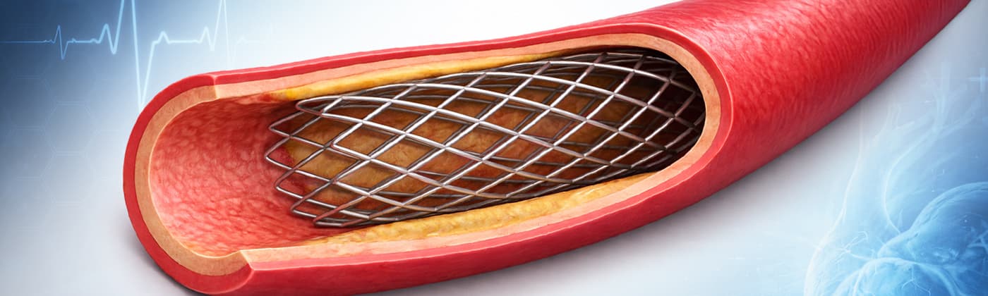
Blood is carried through arteries from the heart to the rest of the body. Any weakening or blockage of these vessels can pose significant health risks and may become life-threatening. A stent is a small mesh tube inserted into the lumen of a blood vessel to treat narrowed or weakened arteries. Stent implantation is now a widely used procedure to support the arterial wall and restore blood flowᶦ.

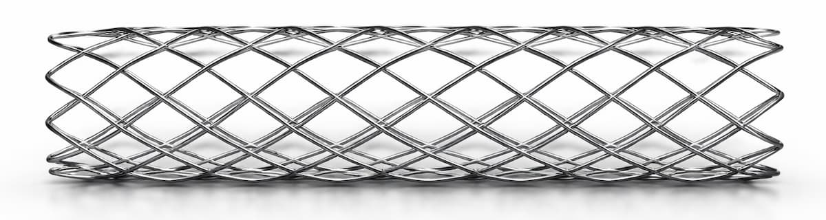
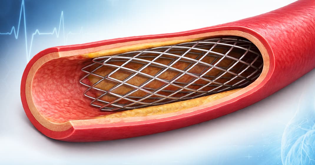
Metal stent mesh geometry illustrating the structural complexity of vascular implant design.

Why coating adhesion matters in drug-eluting stents

Drug-eluting stents represent a major advancement in stent technology. They incorporate a biodegradable, biocompatible polymer coating that enables controlled drug release at the arterial site, helping to inhibit intimal thickening and reduce the risk of restenosisᶦᶦ.

A critical concern in these systems is the delamination of the polymer coating from the metallic stent substrate. This coating carries the drug-eluting layer, and its adhesion directly impacts device performance and reliability.

To improve coating adhesion, stents are often designed with complex geometries. In this study, the polymer coating is located at the bottom of grooves within the stent mesh. This configuration presents a significant challenge for adhesion measurement.

A reliable method is required to quantitatively evaluate the interfacial strength between the polymer coating and the metal substrate. The small diameter of the stent mesh, comparable to a human hair, combined with its three-dimensional geometry, requires:

  • ultrafine X-Y positioning accuracy
  • precise control of applied load
  • accurate depth measurement during testing

Measurement Method

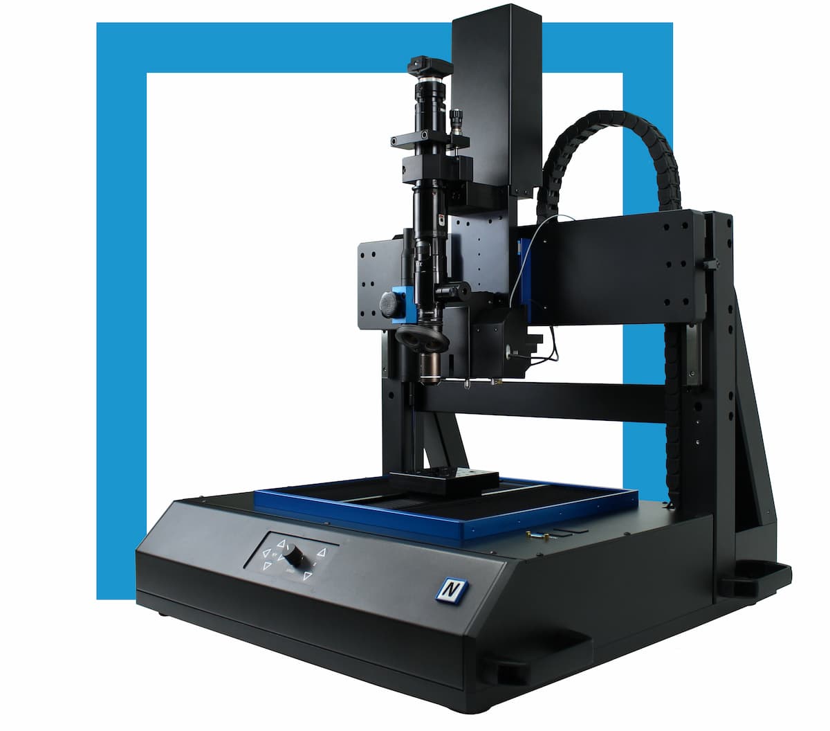
Nano scratch testing is performed using the NANOVEA PB1000 Mechanischer Tester, in Nano Scratch Mode, to evaluate the cohesive and adhesive strength of the polymer coating on the metal mesh of stent samples.

Controlled scratch measurements are carried out on stent geometries with dimensions comparable to a human hair, enabling precise evaluation of coating adhesion on complex stent structures.

NANOVEA PB1000 Advanced

Mechanischer Tester

Testbedingungen

1. Regular Stent Samples

The stent is fixed on the sample stage, with a support wire inserted inside the stent tube to ensure stability during nano scratch testing. The NANOVEA Mechanical Tester is used to perform nano scratch measurements using the parameters summarized in Table 1, to evaluate the cohesive and adhesive strength of the polymer coating on the metal substrate.

ParameterValue
Load typeProgressiv
Initial load0.05 mN
Final load300 and 100 mN
Sliding speed0.5 mm/min
Sliding distance0.5 mm
Indenter geometryKonisch
Indenter material (tip)Diamant
Radius der Eindringkörperspitze20 µm
Temperatur24°C (room)

Tabelle 1: Test parameters for nano scratch measurements on regular stent samples

2. Grooved Stent Samples

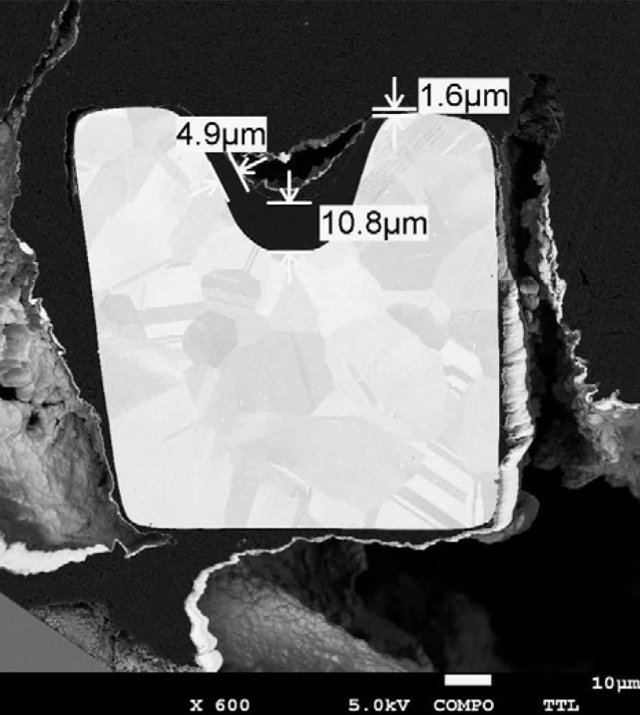
The SEM image in Fig. 1 shows the cross-section of the stent sample. The stent features a groove with a depth of approximately 30 µm. The polymer coating, with a thickness of 10.8 µm, is located at the bottom of the groove.

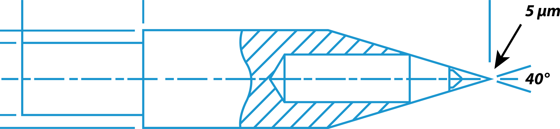
Standard 60° conical diamond tips are not sharp enough to reach the bottom of the groove without contacting the sidewalls. Therefore, a sharper 40° conical diamond tip is used in this study (Fig. 2).

Nano scratch measurements are performed using the parameters summarized in Table 2.

Parameter Value
Load type Progressiv
Initial load 0.1 mN
Final load 300 mN
Ladegeschwindigkeit 300 mN/min
Scratch length 0.25 mm
Scratch speed 0.25 mm/min
Indenter geometry 40° cone
Indenter material (tip) Diamant
Radius der Eindringkörperspitze 5 µm

Table 2: Test parameters for nano scratch measurements on grooved stent samples

stent groove cross section polymer coating thickness adhesion analysis nano scratch testing

Fig. 1: SEM cross-section of a grooved stent showing polymer coating located at the bottom of the groove, highlighting the challenge of coating adhesion measurement in recessed geometries.

nano scratch diamond tip 40 degree stent groove coating adhesion testing schematic

Fig. 2: Schematic of a 40° conical diamond tip designed for nano scratch testing inside stent grooves, enabling accurate adhesion measurement without sidewall interference.

Ergebnisse und Diskussion

The stent mesh has a diameter of approximately 100 μm, comparable to a human hair. Precise positioning is therefore critical to ensure the scratch test is performed at the center of the stent mesh. The NANOVEA Mechanical Tester provides X–Y positioning accuracy down to 0.25 μm, enabling accurate test placement under the integrated optical microscope.

1. Regular Stent Samples

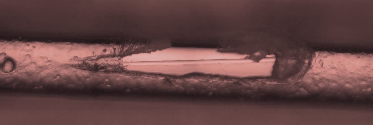
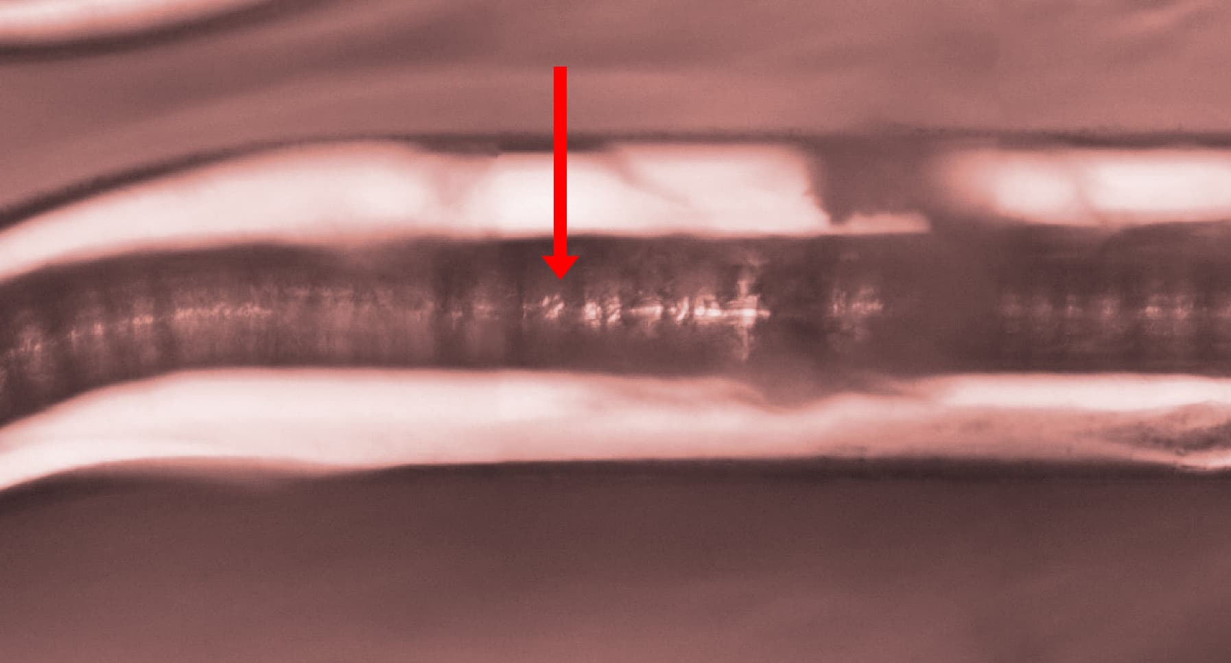
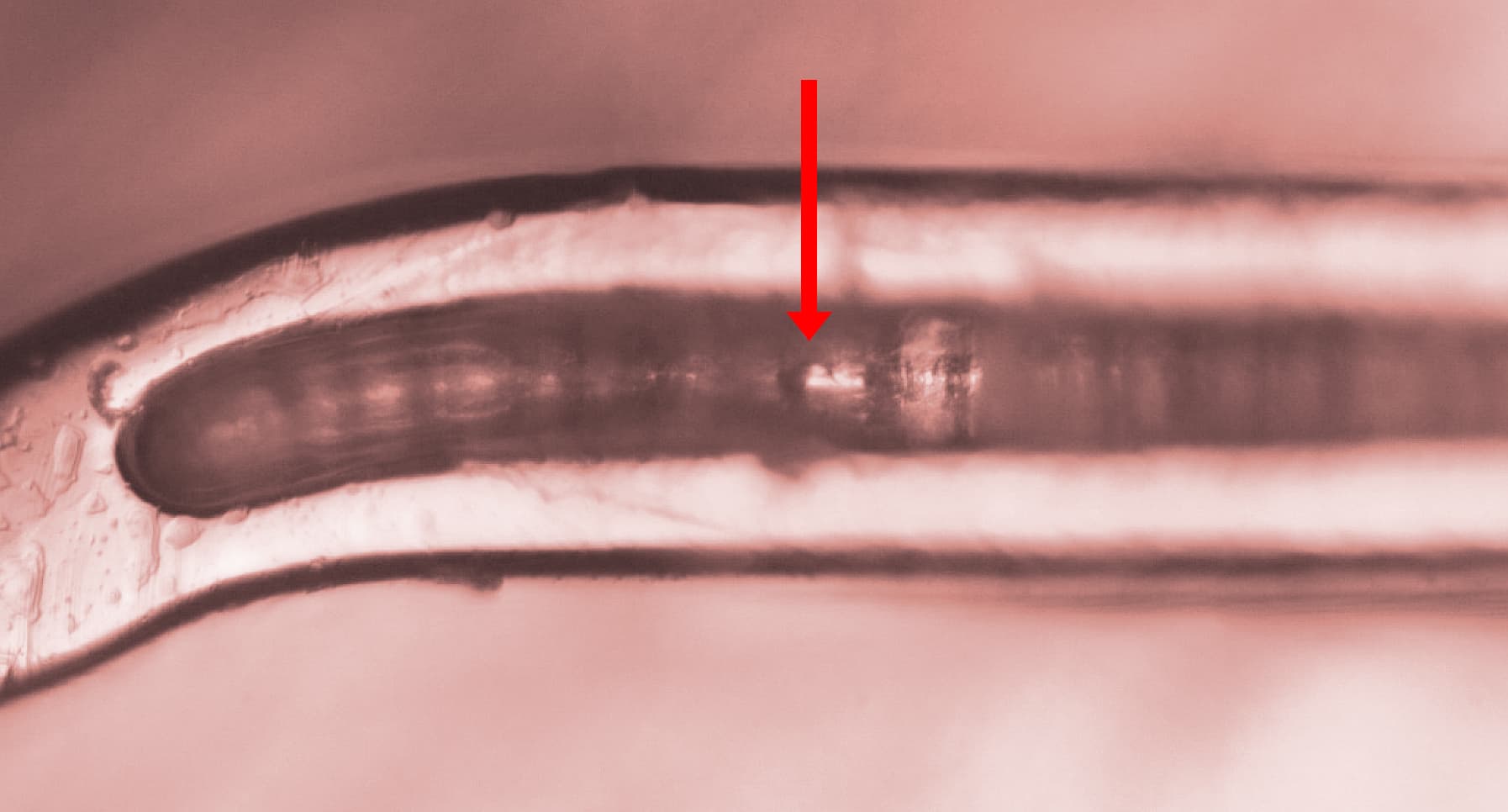
Nano scratch testing is performed with a progressively increasing load up to 300 mN. The full scratch track on the stent is shown in Fig. 3a, while failure behavior at different stages is presented in Fig. 3b and 3c.

Two critical loads are identified:

  • Lc1: the load at which the first visible damage appears on the coating
  • Lc2: the load at which the coating is fully removed and the substrate is exposed

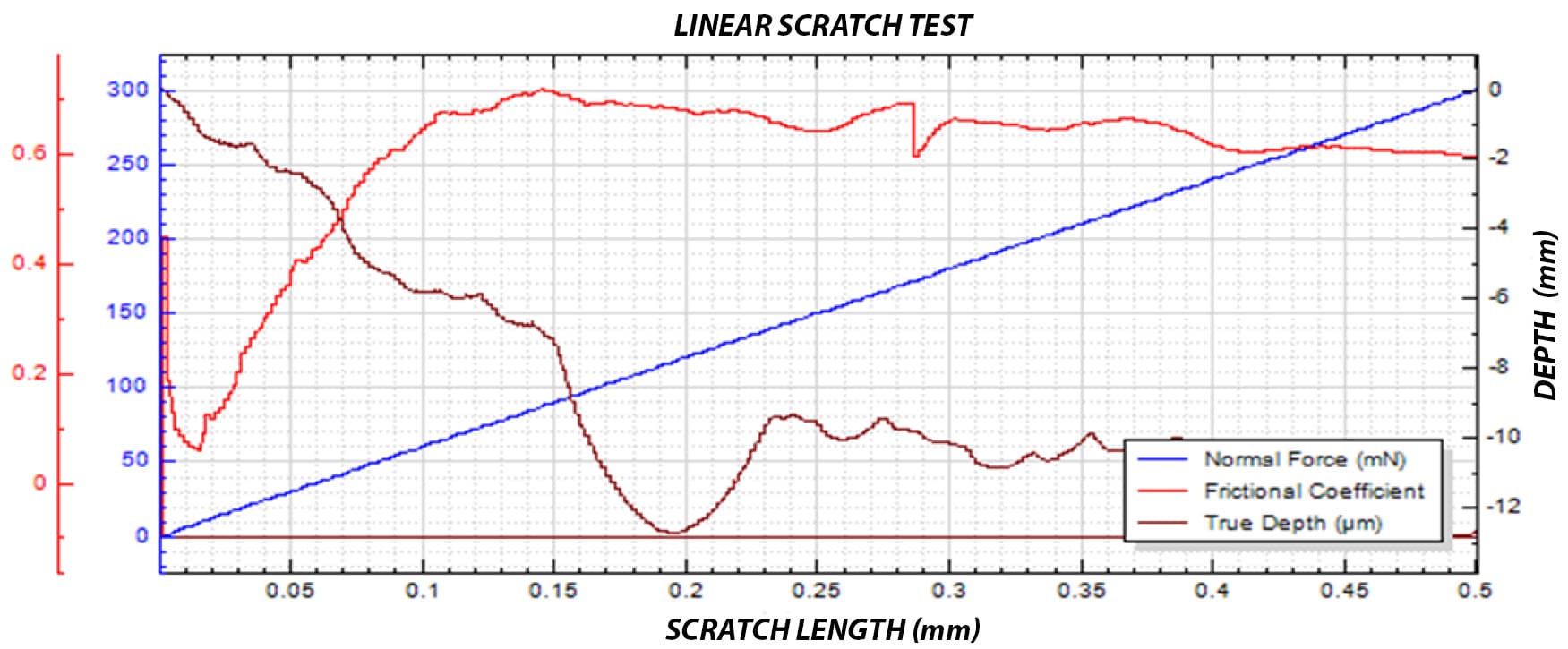
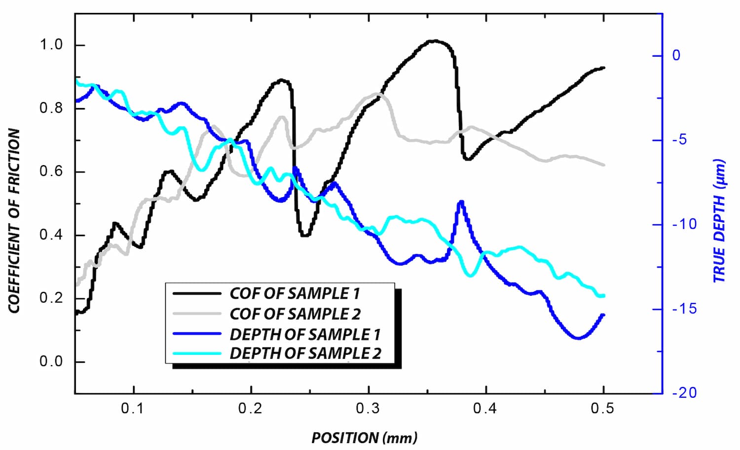
The evolution of coefficient of friction (COF) and penetration depth is shown in Fig. 4, providing insight into the progression of coating failure during the test.

The first signs of coating damage appear at Lc1 ≈ 14.5 mN. As the applied load increases, the diamond tip progressively penetrates the polymer coating, resulting in a wider and deeper scratch track. During this phase, the COF increases from approximately 0.05 to 0.7.

At Lc2 ≈ 78.1 mN, the coating is fully delaminated from the metal substrate. Beyond this point, as the load continues to increase, both COF and penetration depth remain relatively stable due to the mechanical support of the underlying metal substrate.

nano scratch track stent coating progressive load adhesion testing

(a) Full Scratch Track

(b) Lc1 ≈ 14.5 mN

stent coating delamination lc2 nano scratch 78.1 mN adhesion testing

(c) Lc2 ≈ 78.1 mN

Fig. 3: Nano scratch track on a stent coating under progressively increasing load, showing (a) full scratch path, (b) initial coating failure at Lc1 ≈ 14.5 mN, and (c) complete coating delamination at Lc2 ≈ 78.1 mN.

nano scratch testing stent coating coefficient of friction depth progression adhesion failure

Fig. 4: Evolution of coefficient of friction (COF) and penetration depth during nano scratch testing of a stent coating under progressively increasing load, showing the progression of coating failure and transition to substrate support.

Failures during nano scratch testing up to a maximum load of 300 mN occur at critical loads below 100 mN. To enable a more quantitative comparison of coating performance, additional tests are performed with a maximum load of 100 mN on two stent samples, referred to as Sample 1 and Sample 2.

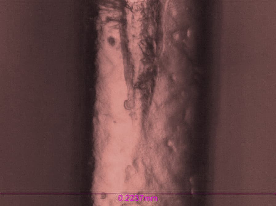
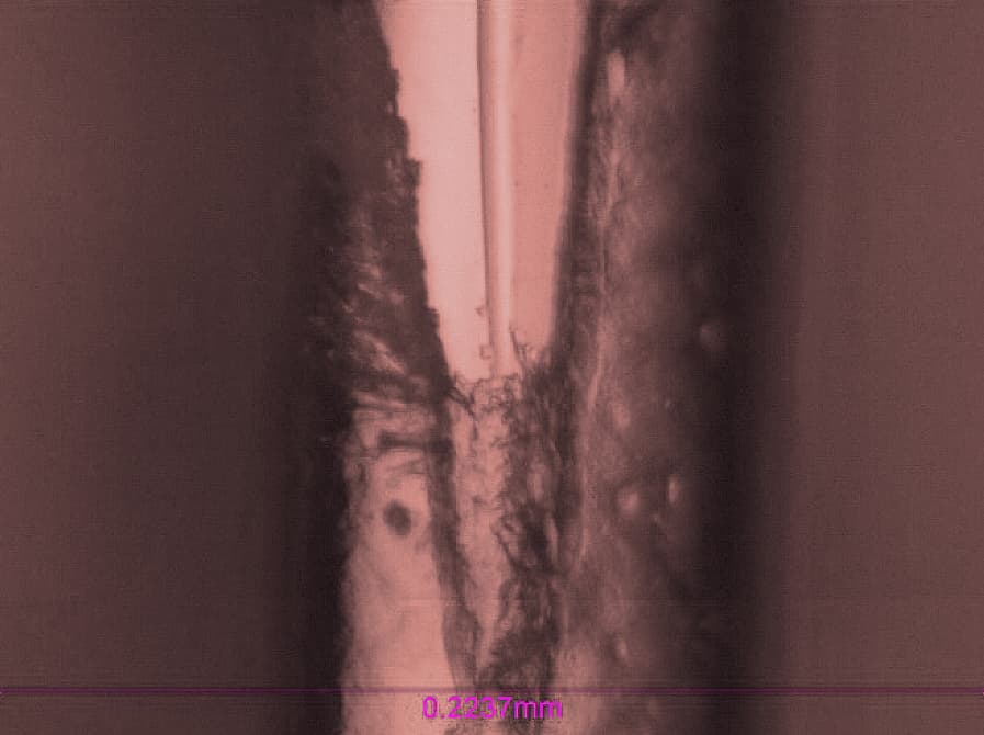
Fig. 5 compares the scratch tracks of Sample 1 and Sample 2 after nano scratch testing. Sample 1 exhibits the first sign of coating damage at a critical load of Lc1 ≈ 13.2 mN, while Sample 2 shows initial failure at a higher load of Lc1 ≈ 21.1 mN.

Coating delamination occurs at 62.5 mN for Sample 1. In contrast, the coating on Sample 2 remains intact throughout the test, continuing to protect the metal substrate under the same loading conditions.

This behavior is further reflected in the evolution of coefficient of friction (COF) and penetration depth, as shown in Fig. 6. When the diamond tip penetrates through the coating and contacts the metal substrate in Sample 1, the COF reaches a peak while the penetration depth decreases due to the increased stiffness of the underlying substrate.

stent coating sample 1 early failure nano scratch track delamination adhesion testing

(a) Sample 1 – Early Coating Failure

stent coating sample 2 high adhesion nano scratch track minimal damage testing

(b) Sample 2 – Improved Coating Integrity

Fig. 5: Comparison of nano scratch tracks for two stent coatings, showing (a) early coating failure and delamination in Sample 1, and (b) improved coating integrity in Sample 2 under the same loading conditions.

nano scratch testing stent coating COF depth comparison sample 1 sample 2 adhesion performance

Fig. 6: Comparison of coefficient of friction (COF) and penetration depth for Sample 1 and Sample 2 during nano scratch testing, showing earlier substrate contact and higher friction response in Sample 1, indicating weaker coating adhesion.

2. Grooved Stent Samples

As shown in Fig. 1 and Fig. 7, the grooved stent mesh has a diameter of approximately 90 μm, comparable to a human hair. The groove has a width of ~50 μm and a depth of 30 μm. This geometry presents a significant challenge for nano scratch testing, particularly for evaluating coating adhesion at the bottom of the groove.

Precise positioning is critical to locate the scratch test within the groove. The nano scratch test is performed with a progressively increasing load up to 300 mN. The full scratch tracks of grooved stent Samples 3 and 4 are compared in Fig. 7.

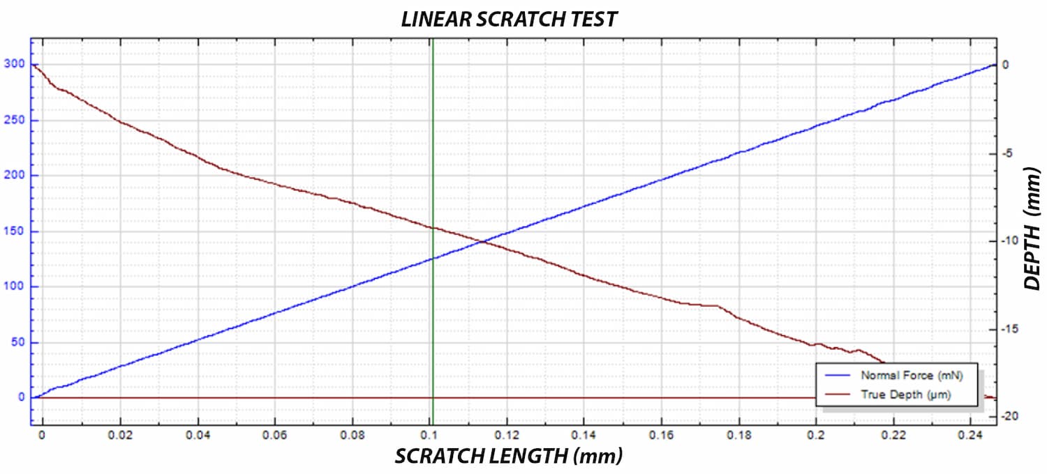
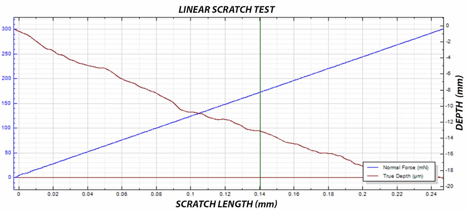
The critical load Lc is defined as the load at which the coating fails and the substrate becomes exposed. The evolution of normal load and penetration depth, shown in Fig. 8, provides further insight into the progression of coating failure during testing.

As the applied load increases, the diamond tip progressively penetrates the polymer coating, resulting in a deeper scratch track. When the critical load Lc is reached, the coating delaminates from the metal substrate.

Sample 3 exhibits coating failure at Lc ≈ 126 mN, while Sample 4 fails at a higher load of Lc ≈ 173 mN. This difference indicates stronger adhesion of the coating in Sample 4.

The measured critical loads enable quantitative comparison of coating adhesion performance. Under the same testing conditions, the coating on Sample 4 demonstrates higher resistance to delamination, making it the better-performing candidate in this study.

stent groove coating failure sample 3 nano scratch 126 mN adhesion testing

(c) Sample 3 – Coating Failure in Groove (Lc ≈ 126 mN)

stent groove coating adhesion sample 4 nano scratch 173 mN minimal failure testing

(d) Sample 4 – Higher Adhesion in Groove (Lc ≈ 173 mN)

Fig. 7: Nano scratch tracks inside stent grooves for Samples 3 and 4, showing (c) coating failure at Lc ≈ 126 mN in Sample 3 and (d) higher adhesion with delayed failure at Lc ≈ 173 mN in Sample 4.

(a) Sample 3 – Earlier Coating Failure (Lc ≈ 126 mN)

(b) Sample 4 – Delayed Failure and Higher Adhesion (Lc ≈ 173 mN)

Fig. 8: Evolution of normal load and penetration depth during nano scratch testing inside stent grooves for Samples 3 and 4, showing earlier coating failure in Sample 3 and delayed failure at higher load in Sample 4. The vertical green line indicates the critical load (Lc) where coating delamination occurs.

Schlussfolgerung

This study demonstrates the ability of the NANOVEA Mechanical Tester to quantitatively evaluate the cohesive and adhesive strength of polymer coatings on both regular and grooved stent geometries using nano scratch testing.

The recessed geometry of the stent grooves, approximately 50 μm wide and 30 μm deep, presents a significant challenge for coating adhesion measurement. The high X–Y positioning accuracy of 0.25 μm enables precise placement of the scratch test within these confined regions, allowing direct evaluation of coating performance where failure is most critical.

By applying a controlled, progressively increasing load, critical loads associated with coating failure can be identified and compared across samples. This approach enables reliable differentiation of coating adhesion performance and interfacial integrity, even on small, complex stent structures.

Referenzen

[I] http://www.nhlbi.nih.gov/health/health-topics/topics/stents
[II] http://www.scielo.org.mx/scielo.php?script=sci_arttext&pid=S1405-99402006000300008

Frequently Asked Questions About Stent Coating Adhesion Testing

What is stent coating adhesion testing?

Stent coating adhesion testing evaluates how strongly a polymer coating is bonded to the metal substrate of a stent. Techniques such as nano scratch testing quantify the load at which coating damage and delamination occur, providing measurable indicators of adhesion strength.

What is critical load (Lc) in nano scratch testing?

Critical load (Lc) is the applied load at which a coating fails during a scratch test.

  • Lc1 corresponds to the first visible damage in the coating
  • Lc2 indicates complete coating removal and exposure of the substrate

These values are used to quantify and compare coating adhesion performance.

Why is coating adhesion important in drug-eluting stents?

Coating adhesion directly affects the reliability of drug-eluting stents. Poor adhesion can lead to coating delamination, which may compromise controlled drug release and increase the risk of device failure.

How do you measure coating adhesion inside stent grooves?

Measuring adhesion inside stent grooves requires high positioning accuracy and appropriate indenter geometry. Nano scratch testing with sharp diamond tips allows access to recessed coating regions, enabling direct evaluation of adhesion within complex stent geometries.

What does coefficient of friction (COF) indicate in scratch testing?

The coefficient of friction (COF) reflects changes in surface interaction during the scratch test. A sudden increase in COF often indicates coating failure and contact between the indenter and the underlying metal substrate.

How can nano scratch testing compare different coating formulations?

Nano scratch testing enables direct comparison of coatings by measuring critical loads under controlled conditions. Higher critical loads indicate stronger adhesion and improved resistance to delamination, allowing selection of better-performing coating systems.

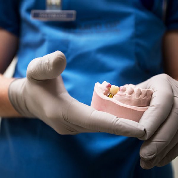
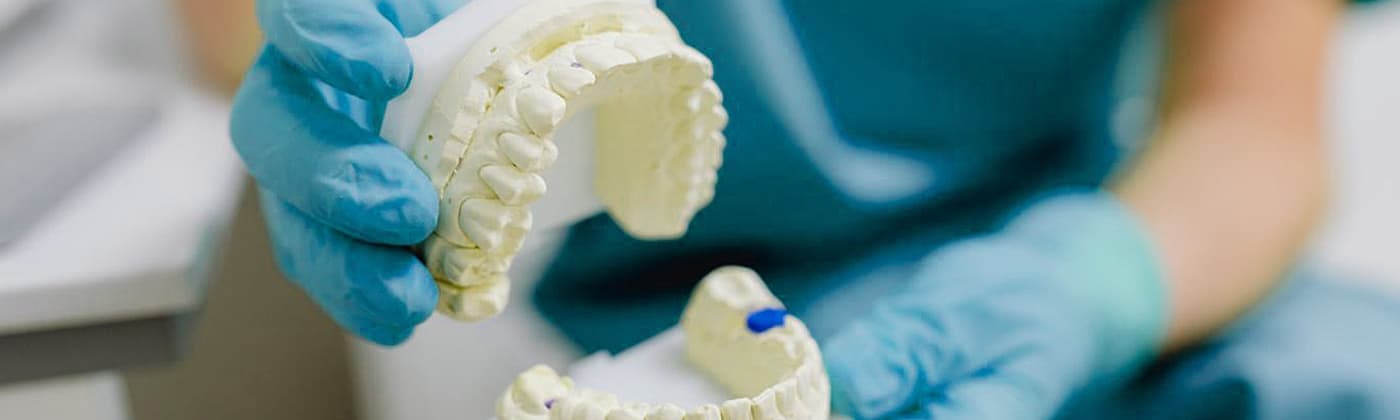
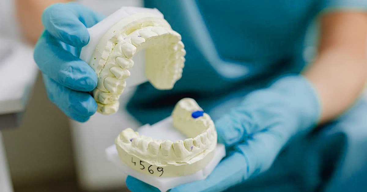
Dentist holding dental model for tooth surface roughness analysis and 3D reconstruction

Dental Surface Roughness Measurement & 3D Tooth Topography

Application Note | Dental Surface Characterization

Dental Surface Roughness Measurement and Full 3D Tooth Topography

Surface Roughness Analysis Using Non-Contact Optical Profilometry

Dental surface roughness measurement and 3D molar reconstruction using optical profilometry

Vorbereitet von

Walter Alabiso, PhD; Davide Morrone, MPhys; Andrew Shore, MA

Einführung

The ability to accurately characterize tooth surfaces, including micro-roughness and 3D surface topography at the nanometer scale, enables advanced research and applications in orthodontics and dental materials science. Non-contact optical profilometry provides a precise method for measuring dental surface roughness and analyzing tooth surface morphology without damaging delicate structures. These measurements support the development of composite dental materials that replicate the natural surface roughness of enamel, as well as the design and fabrication of patient-specific dental casts and restorative components.

Low surface roughness plays a primary role in limiting bacterial adhesion and plaque formation, thereby reducing the risk of cavities. An increase in average roughness (Ra) above 2 µm leads to a steep increase in biofilm formation in vivo.¹ An Ra of 0.2 µm is considered the threshold value below which no further reduction in bacterial adhesion can be expected.²

Reconstruction of the tooth’s 3D surface topography enables the fabrication of dental casts, which are essential for accurate diagnosis, treatment planning, and the fabrication of dental appliances.

Non-Contact Optical Profilometry for Dental Surface Analysis

The present study illustrates the potential of NANOVEA’s high-precision non-contact optical profilometers for dental surface roughness measurement and 3D tooth topography analysis. Chromatic Light technology offers significant advantages over classical touch probe techniques. It acquires data points from deep crevices and complex geometries without introducing measurement errors or artifacts caused by local plastic deformation and without requiring extensive data manipulation.

Compared to focus variation systems, single-point optical sensing provides superior lateral and height accuracy, with X/Y resolution below 0.5 µm, maximum vertical resolution of 1.9 nm, and the ability to measure surface angles up to 87°. The technique is effective on transparent, opaque, specular, diffusive, polished, and rough dental surfaces, making it well suited for comprehensive dental surface characterization.

Measurement Method

Bei dieser Anwendung ist die NANOVEA JR25 Non-Contact Optical Profiler was used to analyze the surface roughness and 3D surface topography of an adult human molar previously affected by tooth decay. The side of the tooth was scanned using a PS2–MG140 single-point optical sensor to measure surface roughness parameters over a defined region of interest and along multiple line profiles.

The crown of the tooth was then scanned and reconstructed using a PS5–MG35 single-point optical sensor, which is suited for larger-area acquisition and full 3D tooth topography measurement.


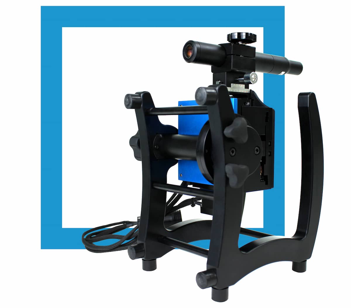
NANOVEA JR25 Portable
Optisches Profilometer

Surface Measurement Using NANOVEA Optical Profilometer

Surface roughness measurements were performed on the lateral side of the molar crown, followed by full 3D reconstruction of the crown surface. Separate single-point optical sensors were used to optimize measurement accuracy for both localized roughness analysis and large-area surface topography acquisition.

PS2 – MG140

Surface roughness analysis by area and parallel line profiles on the side of the tooth’s crown.

PS5 – MG35

Full 3D surface reconstruction of the tooth’s crown.

Messparameter

The following measurement parameters were used for localized surface roughness analysis and full 3D surface reconstruction of the molar crown using NANOVEA single-point optical sensors.

ParameterRoughness Analysis (Area)Roughness Analysis (Profiles)Full 3D Reconstruction
Optical PenPS2-MG140PS2-MG140PS5-MG35
Z-Range [µm]30030010000
X-Distance [mm]2.003.007.50
X-Step Size [µm]1.701.7010.00
Y-Distance [mm]2.001.007.00
Y-Step Size [µm]1.70100.0010.00
Averaging (Avg)111
Measurement TypeDirectDirectDirect
Acquisition ModeSingle FrequencySingle FrequencyDual Frequency
Acquisition Rate [Hz]200200100–400
Light Intensity [%]100100100

Optical Profilometry Results

Yellow Grip Sample

Surface Roughness Analysis

The image below shows a full 3D rendering of the yellow block’s surface.

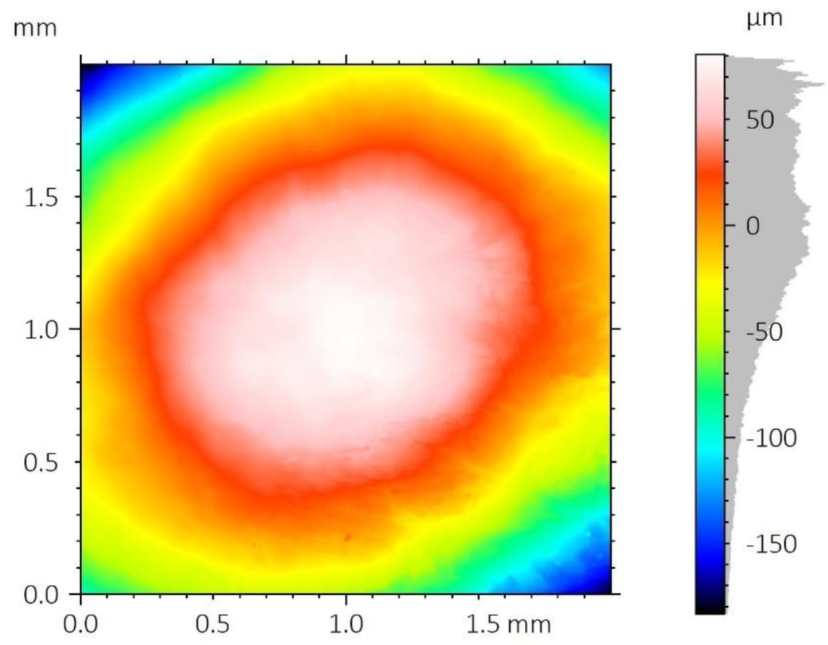
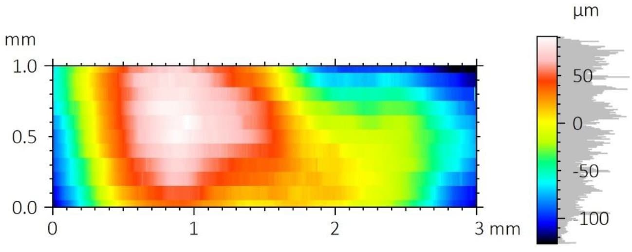
False-color 2D height map of scanned tooth surface region

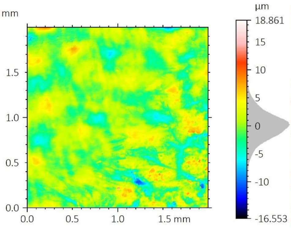
A least-squares degree-8 polynomial form removal was applied to isolate the surface roughness component. The roughness filters S-Gaussian 2.5 µm and L-Gaussian 0.8 mm were then applied according to ISO 25178. The resulting filtered surface and corresponding roughness parameters are presented below.

ISO 25178 – Roughness (S-L)
S-filter (λs): Gaussian, 2.5 µm
F: [Workflow] Form removed (LS-poly 8)
L-filter (λc): Gaussian, 0.8 mm
Height Parameters
Sq2.433µmWurzel-Mittel-Quadrat-Höhe
Ssk-0.102 Schrägheit
Sku3.715 Kurtosis
Sp18.861µmMaximale Peakhöhe
Sv16.553µmMaximum pit depth
Sz35.414µmMaximale Höhe
Sa1.888µmArithmetisches Mittel der Höhe

The average surface roughness Sa is 1.888 µm, while the peak-to-valley height Sz reaches 35.414 µm.

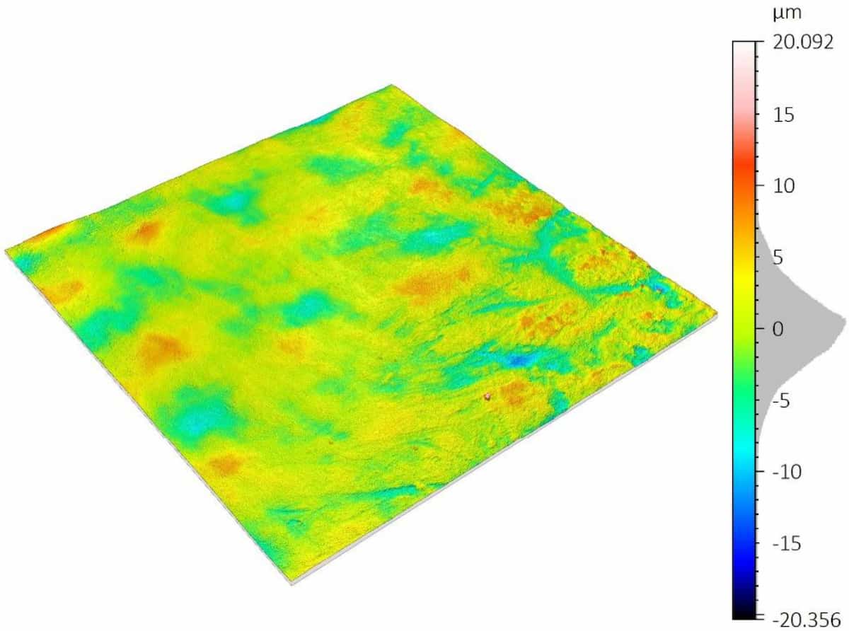
A 3D surface rendering of the filtered area is shown below for visualization.

3D rendering of ISO 25178 filtered tooth surface roughness

Roughness Analysis (Profiles)

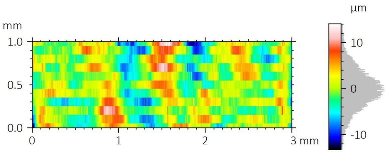
Surface roughness profiles were measured using a series of 11 parallel line scans along the X direction on the side of the tooth. The false-color 2D surface map of the raw scan is shown below.

False-color 2D raw scan of tooth surface for line roughness profiles

The surface form was removed using a least-squares 8-degree polynomial prior to applying the metrological filters, leaving the residual surface shown below.

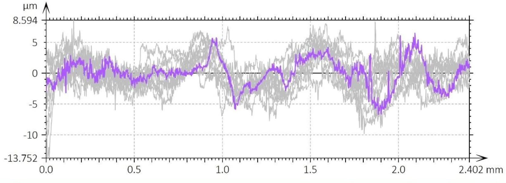
A statistical analysis of the measured surface roughness profiles reveals the following line roughness parameters.

Overlay of multiple tooth surface roughness profiles for statistical analysis

ISO 4287 – Roughness (S-L)
F: Keiner
S-filter (λs): Gaussian, 2.5 µm
L-filter (λc): Gaussian, 0.8 mm
Evaluation length: All λc (3)
Amplitude Parameters – Roughness Profile
  DescriptionMeanStd devMinMax
RpµmMaximum peak height of the roughness profile5.6830.7614.3156.610
RvµmMaximum valley depth of the roughness profile6.2421.0094.7018.438
RzµmMaximum height of roughness profile11.9251.6769.12315.048
RaµmArithmetic mean deviation of the roughness profile2.0630.2971.7102.629
RqµmRoot-mean-square (RMS) deviation of the roughness profile2.5230.3612.0573.175

ISO 4287 – Roughness (S-L)
F: Keiner
S-filter (λs): Gaussian, 2.5 µm
L-filter (λc): Gaussian, 0.8 mm
Evaluation length: All λc (3)
Amplitude Parameters – Roughness Profile
Rpµm
Maximum peak height of the roughness profile
Mean5.683
Std dev0.761
Min4.315
Max6.610
Rvµm
Maximum valley depth of the roughness profile
Mean6.242
Std dev1.009
Min4.701
Max8.438
Rzµm
Maximum height of roughness profile
Mean11.925
Std dev1.676
Min9.123
Max15.048
Raµm
Arithmetic mean deviation of the roughness profile
Mean2.063
Std dev0.297
Min1.710
Max2.629
Rqµm
Root-mean-square (RMS) deviation of the roughness profile
Mean2.523
Std dev0.361
Min2.057
Max3.175

The value of Ra is consistent with the Sa value extracted from the surface area measurement.

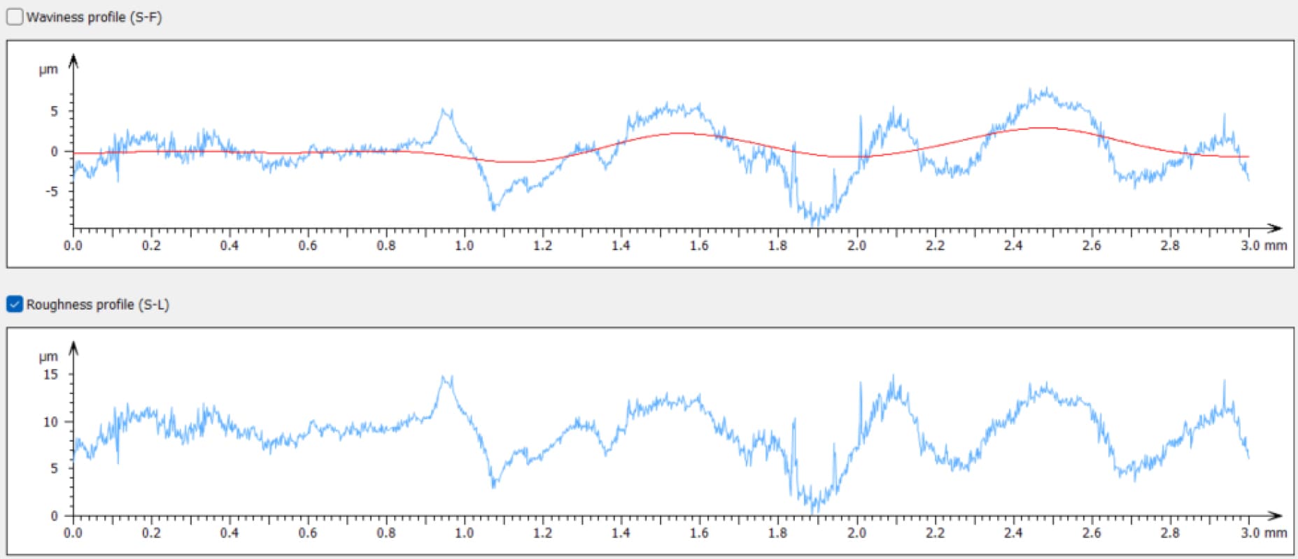
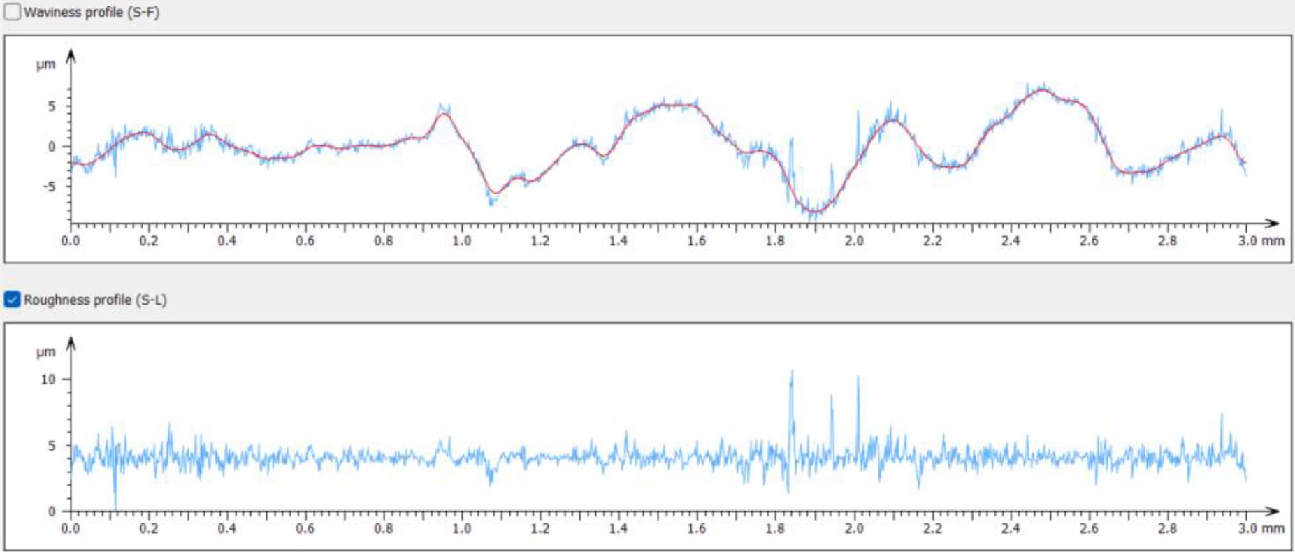
Different metrological filters can be applied to distinguish between macroscopic waviness and microscopic surface roughness. For example, a coarser filter cut-off, such as the 8 mm cut-off used with the Robust Gaussian order-2 filter, produces a smoother waviness profile (red) that is less sensitive to sharp local variations and follows the original surface profile more loosely.

Comparison of waviness and roughness profiles on tooth surface using coarse filter

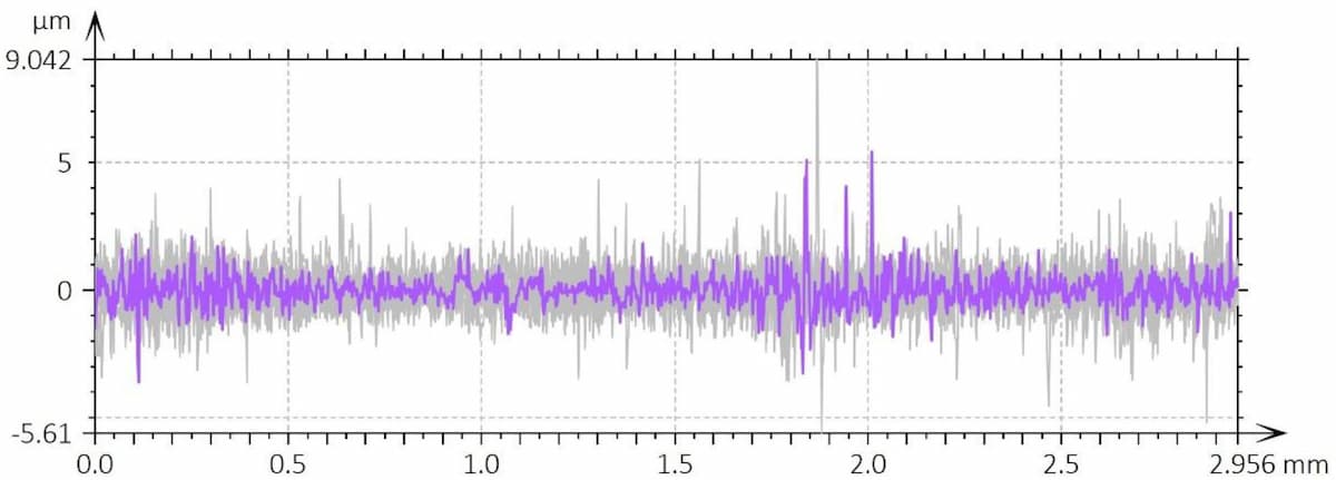
Alternatively, a finer cut-off (e.g., 0.08 mm) enables the analysis of micro-roughness by removing the waviness component that follows the original profile at a larger scale, leaving the finer surface roughness features of the tooth visible.

The microroughness analysis obtained using a 0.08 mm L-Gaussian filter is presented below.

Final microroughness profile of tooth surface after filtering

ISO 4287 – Roughness (S-L)
F: Keiner
S-filter (λs): Gaussian, 2.5 µm
L-filter (λc): Gaussian, 0.08 mm
Evaluation length: All λc (37)
Amplitude Parameters – Roughness Profile
  DescriptionMeanStd devMinMax
RpµmMaximum peak height of the roughness profile1.5820.1221.3421.748
RvµmMaximum valley depth of the roughness profile1.4660.1191.2541.661
RzµmMaximum height of roughness profile3.0490.1962.8203.409
RaµmArithmetic mean deviation of the roughness profile0.4950.0470.4230.597
RqµmRoot-mean-square (RMS) deviation of the roughness profile0.6430.0560.5620.762

ISO 4287 – Roughness (S-L)
F: Keiner
S-filter (λs): Gaussian, 2.5 µm
L-filter (λc): Gaussian, 0.8 mm
Evaluation length: All λc (3)
Amplitude Parameters – Roughness Profile
Rpµm
Maximum peak height of the roughness profile
Mean5.683
Std dev0.761
Min4.315
Max6.610
Rvµm
Maximum valley depth of the roughness profile
Mean6.242
Std dev1.009
Min4.701
Max8.438
Rzµm
Maximum height of roughness profile
Mean11.925
Std dev1.676
Min9.123
Max15.048
Raµm
Arithmetic mean deviation of the roughness profile
Mean2.063
Std dev0.297
Min1.710
Max2.629
Rqµm
Root-mean-square (RMS) deviation of the roughness profile
Mean2.523
Std dev0.361
Min2.057
Max3.175

Full 3D Tooth Surface Topography Reconstruction

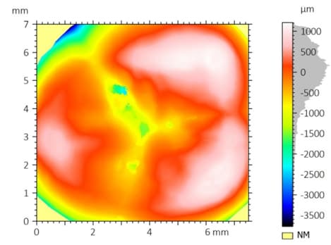
The extended Z-scan range of the PS5 optical sensor enables high-fidelity scanning of the entire tooth crown surface. The resulting 3D surface topography is shown below.

False-color surface topography map of full tooth crown measured with optical profilometer

2D VIEW: 2D surface map of the tooth crown measured with optical profilometry

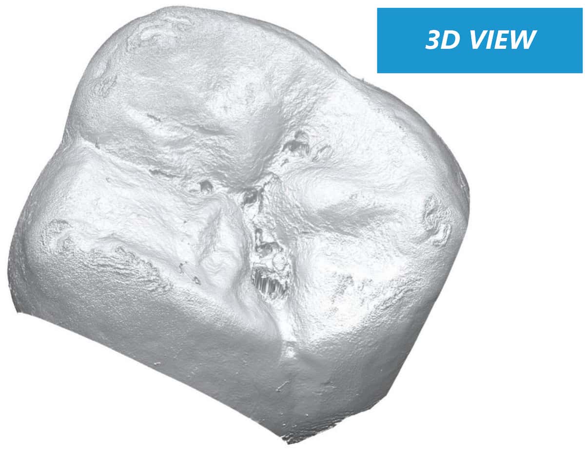
3D surface reconstruction of molar crown from optical profilometer scan

3D VIEW: High-fidelity 3D rendering of the molar crown surface obtained with optical profilometry

Schlussfolgerung

In this application, the NANOVEA JR25 Non-Contact Optical Profiler was used to measure the surface roughness and 3D surface topography of an adult human molar.

Both the area scan and the line profile analysis revealed a roughness Rq of approximately 2.5 µm and an Ra of about 1.9–2.0 µm. These values are consistent with results reported in the literature.³ The use of a narrower L-Gaussian filter with an 80 µm cut-off enabled further investigation of micro-roughness, revealing an Rq of 0.643 µm and an Ra of 0.495 µm.

The full 3D surface topography of the molar crown was reconstructed with high fidelity. The high measurement resolution allows detection of fine surface features and crevices. The resulting surface data can be easily processed and exported as STL files, enabling the design and fabrication of customized dental devices and restorative components.

Referenzen

[1] Shin, B.W., et al. Surface Roughness of Prefabricated Pediatric Zirconia Crowns Following Simulated Toothbrushing. Pediatric Dentistry 44.5 (2022): 363–367.
[2] Bollen, C.M.L., Paul Lambrechts, and Marc Quirynen. Comparison of surface roughness of oral hard materials to the threshold surface roughness for bacterial plaque retention: A review of the literature. Dental Materials 13.4 (1997): 258–269.
[3] Suputtamongkol, K., et al. Surface roughness resulting from wear of lithia-disilicate-based posterior crowns. Wear 269.3–4 (2010): 317–322.

Frequently Asked Questions About Dental Surface Roughness Measurement

What is dental surface roughness measurement?

Dental surface roughness measurement quantifies the microscopic texture of tooth surfaces using parameters such as Ra, Rq, and Sa. Optical profilometers measure these features without contacting the surface, allowing accurate analysis of enamel, restorative materials, and dental crowns.

Why use optical profilometry to measure tooth roughness?

Optical profilometry provides non-contact surface measurement with nanometer-scale vertical resolution. It captures 2D surface maps and full 3D surface topography of dental structures without damaging soft or polished surfaces.

What roughness parameters are used for dental surface analysis?

Common roughness parameters include Ra (arithmetic mean roughness), Rq (root mean square roughness), Sa (areal roughness), and Sz (maximum surface height). These parameters help evaluate enamel wear, plaque adhesion risk, and the performance of restorative materials.

Why is surface roughness important in dentistry?

Surface roughness affects plaque retention, wear resistance, and the long-term performance of dental restorations. Controlling micro-roughness can reduce bacterial adhesion and improve the durability of dental materials.

Need Reliable Surface Roughness Measurement for Dental Materials?

Schweißnahtoberflächeninspektion mit einem tragbaren 3D-Profilometer
WELd-Oberflächeninspektion

Verwendung eines tragbaren 3d-Profilometers

Vorbereitet von

CRAIG LEISING

EINFÜHRUNG

Es kann von entscheidender Bedeutung sein, dass eine bestimmte Schweißnaht, die in der Regel durch eine Sichtprüfung erfolgt, mit einem extremen Präzisionsgrad untersucht wird. Zu den spezifischen Bereichen, die für eine präzise Analyse von Interesse sind, gehören Oberflächenrisse, Porosität und ungefüllte Krater, unabhängig von den nachfolgenden Prüfverfahren. Schweißnahtmerkmale wie Abmessungen/Form, Volumen, Rauheit, Größe usw. können zur kritischen Bewertung gemessen werden.

BEDEUTUNG DES BERÜHRUNGSLOSEN 3D-PROFILOMETERS FÜR DIE SCHWEISSNAHTOBERFLÄCHENPRÜFUNG

Im Gegensatz zu anderen Techniken wie Touch Probes oder Interferometrie bietet die NANOVEA Berührungsloses 3D-ProfilometerMithilfe des axialen Chromatismus kann nahezu jede Oberfläche gemessen werden, die Probengröße kann aufgrund der offenen Bereitstellung stark variieren und es ist keine Probenvorbereitung erforderlich. Der Nano- bis Makrobereich wird während der Oberflächenprofilmessung ohne Einfluss des Probenreflexionsvermögens oder der Probenabsorption erzielt, verfügt über eine erweiterte Fähigkeit zur Messung großer Oberflächenwinkel und es gibt keine Softwaremanipulation der Ergebnisse. Messen Sie ganz einfach jedes Material: transparent, undurchsichtig, spiegelnd, diffus, poliert, rau usw. Die 2D- und 2D-Funktionen der tragbaren NANOVEA-Profilometer machen sie zu idealen Instrumenten für die vollständige Inspektion von Schweißoberflächen sowohl im Labor als auch vor Ort.

MESSZIEL

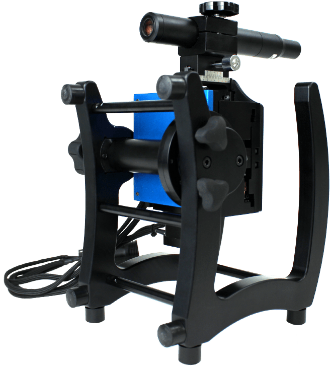
In dieser Anwendung wird der NANOVEA JR25 Portable Profiler verwendet, um die Oberflächenrauheit, die Form und das Volumen einer Schweißnaht sowie die Umgebung zu messen. Diese Daten können wichtige Informationen liefern, um die Qualität der Schweißnaht und des Schweißprozesses richtig zu untersuchen.

NANOVEA

JR25

TESTERGEBNISSE

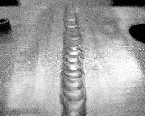
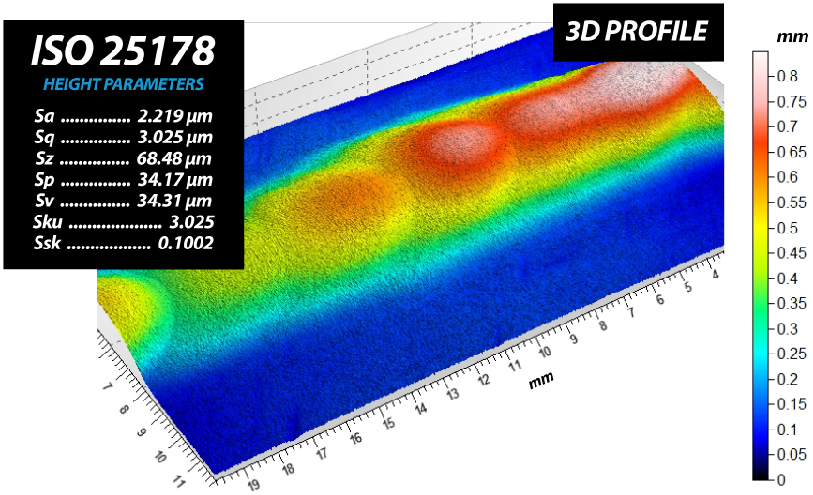
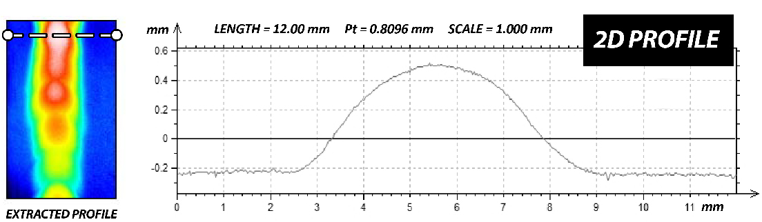
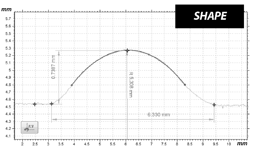
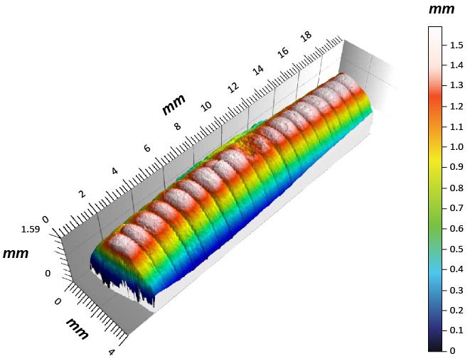
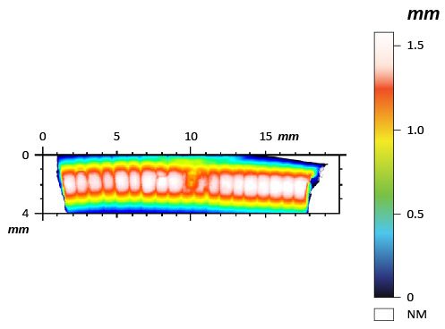
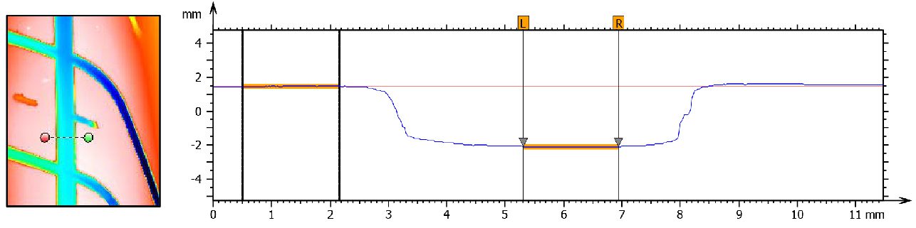
Das Bild unten zeigt die vollständige 3D-Ansicht der Schweißnaht und des umgebenden Bereichs zusammen mit den Oberflächenparametern der Schweißnaht. Das 2D-Querschnittsprofil ist unten dargestellt.

die Probe

Mit dem obigen 2D-Querschnittsprofil, das aus dem 3D-Profil entfernt wurde, werden die Dimensionsinformationen der Schweißnaht unten berechnet. Oberfläche und Volumen des Materials werden nur für die Schweißnaht berechnet.

 HOLEPEAK
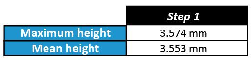
OBERFLÄCHE1,01 mm214,0 mm2
VOLUME8,799e-5 mm323,27 mm3
MAXIMALE TIEFE/HÖHE0,0276 mm0,6195 mm
MITTLERE TIEFE/HÖHE 0,004024 mm 0,2298 mm

SCHLUSSFOLGERUNG

In dieser Anwendung haben wir gezeigt, wie der berührungslose 3D-Profiler NANOVEA kritische Eigenschaften einer Schweißnaht und der sie umgebenden Oberfläche präzise charakterisieren kann. Anhand der Rauheit, der Abmessungen und des Volumens kann eine quantitative Methode für Qualität und Wiederholbarkeit bestimmt und weiter untersucht werden. Musterschweißnähte, wie das Beispiel in dieser App Note, können mit einem Standard-Tischgerät oder einem tragbaren NANOVEA Profiler für Inhouse- oder Feldtests leicht analysiert werden.

Fraktographie-Analyse mit 3D-Profilometrie

FRAKTOGRAPHIE-ANALYSE

3D-PROFILOMETRIE VERWENDEN

Vorbereitet von

CRAIG LEISING

EINFÜHRUNG

Unter Fraktographie versteht man die Untersuchung von Merkmalen auf gebrochenen Oberflächen und wurde in der Vergangenheit mittels Mikroskop oder REM untersucht. Abhängig von der Größe des Merkmals werden für die Oberflächenanalyse ein Mikroskop (Makromerkmale) oder ein REM (Nano- und Mikromerkmale) ausgewählt. Beides ermöglicht letztlich die Identifizierung des Frakturmechanismustyps. Obwohl das Mikroskop effektiv ist, weist es klare Einschränkungen auf, und das REM ist in den meisten Fällen, abgesehen von der Analyse auf atomarer Ebene, für die Messung von Bruchflächen unpraktisch und verfügt nicht über eine breitere Einsatzmöglichkeit. Mit Fortschritten in der optischen Messtechnik ist das NANOVEA Berührungsloses 3D-Profilometer gilt heute als das Instrument der Wahl, da es in der Lage ist, 2D- und 3D-Oberflächenmessungen im Nano- bis Makromaßstab durchzuführen

BEDEUTUNG DES BERÜHRUNGSLOSEN 3D-PROFILOMETERS FÜR DIE BRUCHPRÜFUNG

Im Gegensatz zu einem SEM kann ein berührungsloses 3D-Profilometer nahezu jede Oberfläche und Probengröße mit minimaler Probenvorbereitung messen und bietet dabei bessere vertikale/horizontale Abmessungen als ein SEM. Mit einem Profilometer werden Merkmale im Nano- bis Makrobereich in einer einzigen Messung erfasst, ohne dass die Reflektivität der Probe eine Rolle spielt. Sie können problemlos jedes Material messen: transparent, undurchsichtig, spiegelnd, diffus, poliert, rau usw. Das berührungslose 3D-Profilometer bietet umfassende und benutzerfreundliche Funktionen zur Maximierung von Oberflächenbruchstudien zu einem Bruchteil der Kosten eines REM.

MESSZIEL

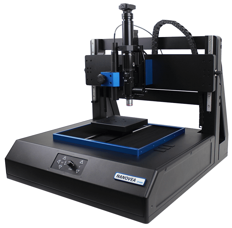
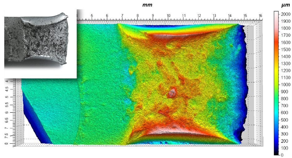
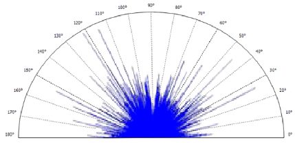
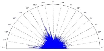
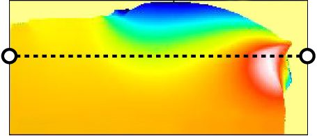
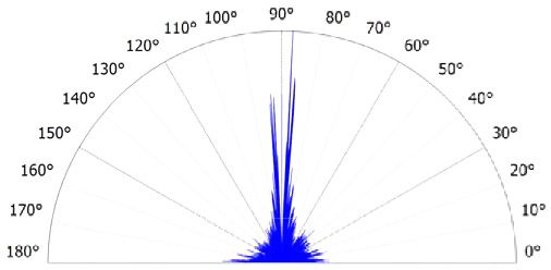
In dieser Anwendung wird das NANOVEA ST400 zur Messung der gebrochenen Oberfläche einer Stahlprobe verwendet. In dieser Studie werden wir eine 3D-Fläche, eine 2D-Profilextraktion und eine Richtungskarte der Oberfläche zeigen.

NANOVEA

ST400

ERGEBNISSE

OBERFLÄCHE

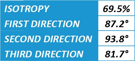
3D-Oberflächentextur Richtung

Isotropie51.26%
Erste Richtung123.2º
Zweite Richtung116.3º
Dritte Richtung0.1725º

Oberfläche, Volumen, Rauheit und viele andere können automatisch aus dieser Extraktion berechnet werden.

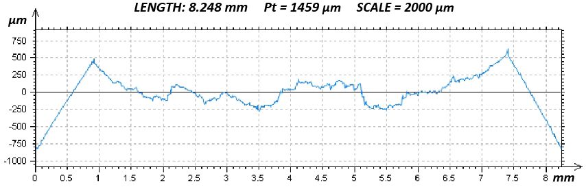
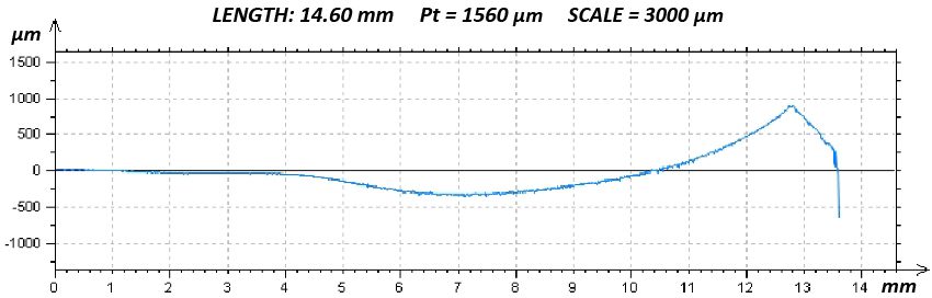
2D-Profil-Extraktion

ERGEBNISSE

SEITENOBERFLÄCHE

3D-Oberflächentextur Richtung

Isotropie15.55%
Erste Richtung0.1617º
Zweite Richtung110.5º
Dritte Richtung171.5º

Oberfläche, Volumen, Rauheit und viele andere können automatisch aus dieser Extraktion berechnet werden.

2D-Profil-Extraktion

SCHLUSSFOLGERUNG

In dieser Anwendung haben wir gezeigt, wie das berührungslose 3D-Profilometer NANOVEA ST400 die gesamte Topografie (Nano-, Mikro- und Makromerkmale) einer gebrochenen Oberfläche präzise charakterisieren kann. Aus dem 3D-Bereich kann die Oberfläche eindeutig identifiziert werden, und Teilbereiche oder Profile/Querschnitte können schnell extrahiert und mit einer endlosen Liste von Oberflächenberechnungen analysiert werden. Oberflächenmerkmale im Subnanometerbereich können mit einem integrierten AFM-Modul weiter analysiert werden.

Darüber hinaus hat NANOVEA eine tragbare Version seines Profilometers entwickelt, die sich besonders für Feldstudien eignet, bei denen die Bruchfläche nicht bewegt werden kann. Mit dieser umfangreichen Liste von Oberflächenmessfunktionen war die Analyse von Bruchflächen noch nie so einfach und bequem mit einem einzigen Gerät.

Polymerriemenverschleiß und Reibung mit einem Tribometer

POLYMER-GURTE

Abnutzung und Reibung mit einem TRIBOMETER

Vorbereitet von

DUANJIE LI, PhD

EINFÜHRUNG

Riemenantriebe übertragen Leistung und verfolgen die Relativbewegung zwischen zwei oder mehr rotierenden Wellen. Als einfache und kostengünstige Lösung mit minimalem Wartungsaufwand sind Riemenantriebe in einer Vielzahl von Anwendungen weit verbreitet, z. B. bei Bügelsägen, Sägewerken, Dreschmaschinen, Silogebläsen und Förderanlagen. Riemenantriebe können die Maschinen vor Überlast schützen sowie Schwingungen dämpfen und isolieren.

BEDEUTUNG DER VERSCHLEISSBEWERTUNG FÜR RIEMENANTRIEBE

Reibung und Verschleiß sind für die Riemen in einer riemengetriebenen Maschine unvermeidlich. Eine ausreichende Reibung sorgt für eine effektive Kraftübertragung ohne Schlupf, aber eine übermäßige Reibung kann den Riemen schnell verschleißen. Während des Betriebs des Riemenantriebs treten verschiedene Arten von Verschleiß auf, wie Ermüdung, Abrieb und Reibung. Um die Lebensdauer des Riemens zu verlängern und die Kosten und den Zeitaufwand für die Reparatur und den Austausch des Riemens zu senken, ist eine zuverlässige Bewertung des Verschleißverhaltens der Riemen wünschenswert, um die Lebensdauer des Riemens, die Produktionseffizienz und die Anwendungsleistung zu verbessern. Die genaue Messung des Reibungskoeffizienten und der Verschleißrate des Riemens erleichtert die Forschung und Entwicklung sowie die Qualitätskontrolle der Riemenproduktion.

MESSZIEL

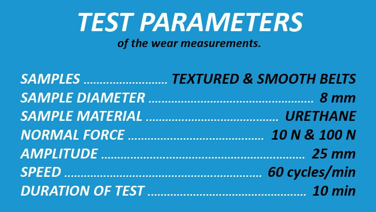
In dieser Studie haben wir das Verschleißverhalten von Riemen mit unterschiedlichen Oberflächenstrukturen simuliert und verglichen, um die Leistungsfähigkeit des Systems zu demonstrieren. NANOVEA T2000 Tribometer bei der kontrollierten und überwachten Simulation des Verschleißprozesses des Riemens.

NANOVEA

T2000

PRÜFVERFAHREN

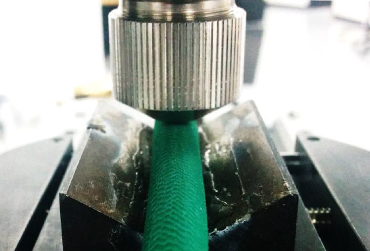
Der Reibungskoeffizient (COF) und die Verschleißfestigkeit von zwei Riemen mit unterschiedlicher Oberflächenrauheit und -struktur wurden mit dem NANOVEA Hohe Belastung Tribometer unter Verwendung des linear hin- und hergehenden Verschleißmoduls. Als Gegenmaterial wurde eine Kugel aus Stahl 440 (10 mm Durchmesser) verwendet. Die Oberflächenrauheit und die Verschleißspur wurden mit einem integrierten Prüfgerät untersucht Berührungsloses 3D-Profilometer. Die Verschleißrate, Kwurde anhand der folgenden Formel bewertet K=Vl(Fxs), wobei V ist das abgenutzte Volumen, F ist die Normalbelastung und s ist die Gleitstrecke.


Bitte beachten Sie, dass in dieser Studie eine glatte 440er Stahlkugel als Beispiel verwendet wurde. Jedes feste Material mit unterschiedlichen Formen und Oberflächenbeschaffenheiten kann mit Hilfe spezieller Vorrichtungen verwendet werden, um die tatsächliche Anwendungssituation zu simulieren.

ERGEBNISSE & DISKUSSION

Der strukturierte Gürtel und der glatte Gürtel haben eine Oberflächenrauhigkeit Ra von 33,5 bzw. 8,7 um, wie aus den analysierten Oberflächenprofilen hervorgeht, die mit einer NANOVEA Berührungsloser optischer 3D-Profiler. Der COF und die Verschleißrate der beiden getesteten Riemen wurden bei 10 N bzw. 100 N gemessen, um das Verschleißverhalten der Riemen bei unterschiedlichen Belastungen zu vergleichen.

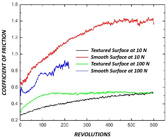
ABBILDUNG 1 zeigt die Entwicklung des COF der Riemen während der Verschleißtests. Die Riemen mit unterschiedlichen Texturen weisen ein deutlich unterschiedliches Verschleißverhalten auf. Interessanterweise erreicht der strukturierte Riemen nach der Einlaufphase, in der der COF allmählich ansteigt, einen niedrigeren COF von ~0,5 in beiden Tests, die mit einer Last von 10 N und 100 N durchgeführt wurden. Im Vergleich dazu weist der glatte Riemen, der mit einer Last von 10 N getestet wurde, einen deutlich höheren COF von ~1,4 auf, wenn der COF stabil wird, und bleibt für den Rest des Tests über diesem Wert. Der mit einer Belastung von 100 N getestete Glattriemen wurde durch die Stahlkugel 440 schnell verschlissen und bildete eine große Verschleißspur. Der Test wurde daher bei 220 Umdrehungen abgebrochen.

ABBILDUNG 1: Entwicklung des COF der Riemen bei unterschiedlichen Belastungen.

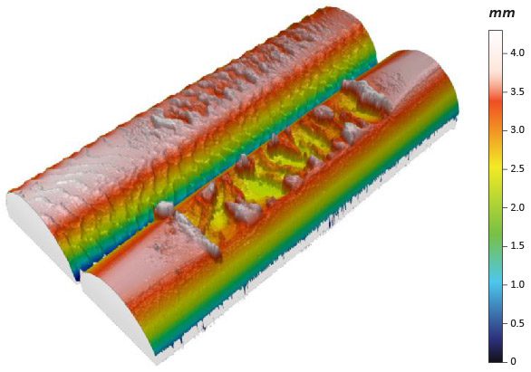
ABBILDUNG 2 vergleicht die 3D-Verschleißspurenbilder nach den Tests mit 100 N. Das berührungslose 3D-Profilometer NANOVEA bietet ein Werkzeug zur Analyse der detaillierten Morphologie der Verschleißspuren, das weitere Einblicke in das grundlegende Verständnis des Verschleißmechanismus ermöglicht.

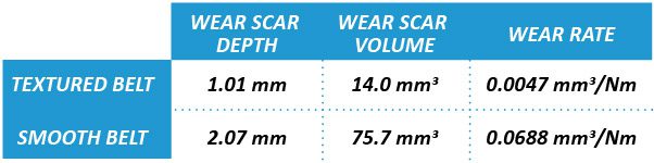
TABELLE 1: Ergebnis der Analyse der Verschleißspuren.

ABBILDUNG 2:  3D-Ansicht der beiden Bänder
nach den Tests bei 100 N.

Das 3D-Verschleißspurprofil ermöglicht eine direkte und genaue Bestimmung des von der fortschrittlichen Analysesoftware berechneten Verschleißspurvolumens, wie in TABELLE 1 dargestellt. Bei einem Verschleißtest mit 220 Umdrehungen weist der Glattriemen eine viel größere und tiefere Verschleißspur mit einem Volumen von 75,7 mm3 auf, während das Verschleißvolumen des Strukturriemens nach einem Verschleißtest mit 600 Umdrehungen 14,0 mm3 beträgt. Die deutlich höhere Reibung des Glattriemens an der Stahlkugel führt zu einer 15-fach höheren Verschleißrate im Vergleich zum strukturierten Riemen.


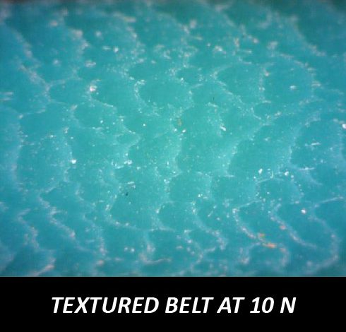
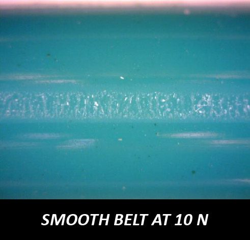
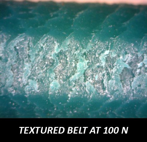
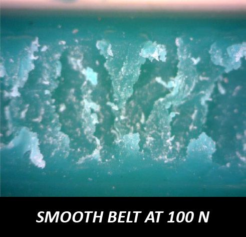
Ein solch drastischer Unterschied der COF zwischen dem strukturierten und dem glatten Gürtel hängt möglicherweise mit der Größe der Kontaktfläche zwischen dem Gürtel und der Stahlkugel zusammen, was auch zu ihrem unterschiedlichen Verschleißverhalten führt. ABBILDUNG 3 zeigt die Verschleißspuren der beiden Riemen unter dem Lichtmikroskop. Die Untersuchung der Verschleißspuren stimmt mit der Beobachtung der COF-Entwicklung überein: Der strukturierte Gurt, der einen niedrigen COF von ~0,5 aufweist, zeigt nach dem Verschleißtest bei einer Belastung von 10 N keine Anzeichen von Verschleiß. Der glatte Gurt zeigt eine kleine Verschleißspur bei 10 N. Die Verschleißtests bei 100 N erzeugen sowohl auf dem strukturierten als auch auf dem glatten Gurt wesentlich größere Verschleißspuren, und die Verschleißrate wird anhand von 3D-Profilen berechnet, wie im folgenden Abschnitt erläutert wird.

ABBILDUNG 3:  Abnutzungsspuren unter dem Lichtmikroskop.

SCHLUSSFOLGERUNG

In dieser Studie haben wir die Fähigkeit des NANOVEA T2000 Tribometers aufgezeigt, den Reibungskoeffizienten und die Verschleißrate von Riemen kontrolliert und quantitativ zu bestimmen. Die Oberflächentextur spielt eine entscheidende Rolle für die Reibung und den Verschleißwiderstand der Riemen während ihres Einsatzes. Der strukturierte Riemen weist einen stabilen Reibungskoeffizienten von ~0,5 auf und besitzt eine lange Lebensdauer, was zu einem geringeren Zeit- und Kostenaufwand für die Reparatur oder den Austausch von Werkzeugen führt. Die übermäßige Reibung des glatten Riemens an der Stahlkugel führt dagegen zu einer schnellen Abnutzung des Riemens. Außerdem ist die Belastung des Riemens ein entscheidender Faktor für seine Lebensdauer. Eine Überlastung erzeugt eine sehr hohe Reibung, die zu einem beschleunigten Verschleiß des Riemens führt.

Das NANOVEA T2000 Tribometer bietet präzise und wiederholbare Verschleiß- und Reibungstests mit ISO- und ASTM-konformen Rotations- und Linearmodi, mit optionalen Modulen für Hochtemperaturverschleiß, Schmierung und Tribokorrosion in einem vorintegrierten System. NANOVEAs unmatched ist die ideale Lösung für die Bestimmung der gesamten Bandbreite tribologischer Eigenschaften von dünnen oder dicken, weichen oder harten Beschichtungen, Filmen und Substraten.

Fossiles Mikrogefüge mit 3D-Profilometrie
FOSSILES GEFÜGE

3D-PROFILOMETRIE VERWENDEN

Vorbereitet von

DUANJIE LI, PhD

EINFÜHRUNG

Fossilien sind die konservierten Überreste von Pflanzen, Tieren und anderen Organismen, die im Sediment unter alten Meeren, Seen und Flüssen vergraben sind. Das weiche Körpergewebe zerfällt normalerweise nach dem Tod, aber die harten Schalen, Knochen und Zähne versteinern. Mikrostrukturelle Oberflächenmerkmale bleiben oft erhalten, wenn die ursprünglichen Schalen und Knochen durch Mineralien ersetzt werden, was Aufschluss über die Entwicklung der Witterung und den Entstehungsmechanismus der Fossilien gibt.

BEDEUTUNG EINES BERÜHRUNGSLOSEN 3D-PROFILOMETERS FÜR DIE UNTERSUCHUNG VON FOSSILIEN

3D-Profile des Fossils ermöglichen es uns, die detaillierten Oberflächenmerkmale der Fossilprobe aus einem näheren Blickwinkel zu betrachten. Die hohe Auflösung und Genauigkeit des NANOVEA-Profilometers sind mit bloßem Auge möglicherweise nicht erkennbar. Die Analysesoftware des Profilometers bietet eine breite Palette von Studien, die auf diese einzigartigen Oberflächen anwendbar sind. Im Gegensatz zu anderen Techniken wie Touch Probes bietet der NANOVEA Berührungsloses 3D-Profilometer Misst die Oberflächenmerkmale, ohne die Probe zu berühren. Dies ermöglicht die Erhaltung der wahren Oberflächenmerkmale bestimmter empfindlicher Fossilienproben. Darüber hinaus ermöglicht das tragbare Profilometer Modell Jr25 3D-Messungen an Fossilienstandorten, was die Fossilanalyse und den Schutz nach der Ausgrabung erheblich erleichtert.

MESSZIEL

In dieser Studie wird das NANOVEA Jr25 Profilometer verwendet, um die Oberfläche von zwei repräsentativen Fossilienproben zu messen. Die gesamte Oberfläche jedes Fossils wurde gescannt und analysiert, um die Oberflächenmerkmale zu charakterisieren, darunter Rauheit, Kontur und Texturrichtung.

NANOVEA

Jr25

FOSSIL EINES BRACHIOPODEN

Die erste fossile Probe, die in diesem Bericht vorgestellt wird, ist ein Brachiopod-Fossil, das von einem Meerestier stammt, das an der Ober- und Unterseite harte "Klappen" (Schalen) hat. Sie traten erstmals im Kambrium auf, das heißt vor mehr als 550 Millionen Jahren.

Die 3D-Ansicht des Scans ist in ABBILDUNG 1 und die Falschfarbenansicht in ABBILDUNG 2 dargestellt. 

ABBILDUNG 1: 3D-Ansicht der fossilen Brachiopodenprobe.

ABBILDUNG 2: Falschfarbenansicht der fossilen Brachiopodenprobe.

Die Gesamtform wurde dann von der Oberfläche entfernt, um die lokale Oberflächenmorphologie und -kontur des Brachiopodenfossils zu untersuchen (siehe ABBILDUNG 3). Auf dem Brachiopoden-Fossil ist nun eine eigentümliche, divergierende Rillentextur zu beobachten.

ABBILDUNG 3: Falschfarbenansicht und Konturlinienansicht nach dem Entfernen der Form.

Aus dem strukturierten Bereich wird ein Linienprofil extrahiert, um eine Querschnittsansicht der fossilen Oberfläche zu zeigen (ABBILDUNG 4). Die Stufenhöhenstudie misst die genauen Abmessungen der Oberflächenmerkmale. Die Rillen weisen eine durchschnittliche Breite von ~0,38 mm und eine Tiefe von ~0,25 mm auf.

ABBILDUNG 4: Studien zum Linienprofil und zur Stufenhöhe der strukturierten Oberfläche.

SEELILIENSTAMM-FOSSIL

Bei der zweiten fossilen Probe handelt es sich um ein Stammfossil einer Seelilie. Stachelhäuter tauchten erstmals in den Meeren des mittleren Kambriums auf, etwa 300 Millionen Jahre vor den Dinosauriern. 


Die 3D-Ansicht des Scans ist in ABBILDUNG 5 und die Falschfarbenansicht in ABBILDUNG 6 dargestellt. 

ABBILDUNG 5: 3D-Ansicht der fossilen Crinoidenprobe.

Die Isotropie der Oberflächentextur und die Rauheit des Crinoiden-Stammfossils werden in ABBILDUNG 7 analysiert. 

 Dieses Fossil weist eine bevorzugte Texturrichtung in einem Winkel nahe 90° auf, was zu einer Isotropie der Textur von 69% führt.

ABBILDUNG 6: Falschfarbenansicht des Stiel einer Seelilie Probe.


ABBILDUNG 7: Isotropie der Oberflächentextur und Rauheit des Stammfossils der Crinoide.

Das 2D-Profil entlang der axialen Richtung des Crinoiden-Stammfossils ist in ABBILDUNG 8 dargestellt. 

Die Größe der Spitzen der Oberflächentextur ist ziemlich einheitlich.

ABBILDUNG 8: 2D-Profilanalyse des Crinoiden-Stammfossils.

SCHLUSSFOLGERUNG

In dieser Anwendung haben wir die 3D-Oberflächenmerkmale eines fossilen Brachiopoden- und Crinoidenstamms mit dem tragbaren berührungslosen Profilometer NANOVEA Jr25 umfassend untersucht. Wir zeigen, dass das Gerät die 3D-Morphologie der fossilen Proben präzise charakterisieren kann. Die interessanten Oberflächenmerkmale und Texturen der Proben werden dann weiter analysiert. Die Brachiopodenprobe weist eine divergente Rillentextur auf, während das Crinoidenstammfossil eine bevorzugte Texturisotropie zeigt. Die detaillierten und präzisen 3D-Oberflächenscans erweisen sich als ideale Werkzeuge für Paläontologen und Geologen, um die Entwicklung des Lebens und die Entstehung von Fossilien zu untersuchen.

Die hier gezeigten Daten stellen nur einen Teil der in der Analysesoftware verfügbaren Berechnungen dar. NANOVEA Profilometer messen praktisch jede Oberfläche in Bereichen wie Halbleiter, Mikroelektronik, Solar, Faseroptik, Automobil, Luft- und Raumfahrt, Metallurgie, Bearbeitung, Beschichtungen, Pharmazeutik, Biomedizin, Umwelt und vielen anderen.

Styropor-Oberflächen-Grenzflächenmessung Profilometrie

Grenzflächenmessung

Grenzflächenmessung mit 3D-Profilometrie

Mehr erfahren

OBERFLÄCHENGRENZFLÄCHENMESSUNG

3D-PROFILOMETRIE VERWENDEN

Vorbereitet von

Craig Leising

EINFÜHRUNG

Bei Studien, in denen die Schnittstelle von Oberflächenmerkmalen, Mustern, Formen usw. zur Orientierung ausgewertet wird, ist es nützlich, schnell Bereiche von Interesse über das gesamte Messprofil zu identifizieren. Durch die Segmentierung einer Oberfläche in signifikante Bereiche kann der Benutzer schnell Grenzen, Spitzen, Vertiefungen, Flächen, Volumina und vieles mehr bewerten, um ihre funktionelle Rolle im gesamten untersuchten Oberflächenprofil zu verstehen. Wie zum Beispiel bei der Korngrenzenabbildung von Metallen ist die Bedeutung der Analyse die Schnittstelle vieler Strukturen und ihre Gesamtausrichtung. Durch das Verständnis jedes einzelnen Bereichs von Interesse können Defekte und Anomalien innerhalb des Gesamtbereichs identifiziert werden. Obwohl die Korngrenzenabbildung in der Regel in einem Bereich untersucht wird, der die Möglichkeiten des Profilometers übersteigt, und es sich nur um eine 2D-Bildanalyse handelt, ist sie eine hilfreiche Referenz, um das Konzept dessen zu veranschaulichen, was hier in größerem Maßstab zusammen mit den Vorteilen der 3D-Oberflächenmessung gezeigt wird.

BEDEUTUNG DES BERÜHRUNGSLOSEN 3D-PROFILOMETERS FÜR DIE UNTERSUCHUNG DER OBERFLÄCHENTRENNUNG

Im Gegensatz zu anderen Techniken wie Touch Probes oder Interferometrie ist die 3D berührungsloses ProfilometerMithilfe des axialen Chromatismus kann nahezu jede Oberfläche gemessen werden, die Probengröße kann aufgrund des offenen Stagings stark variieren und es ist keine Probenvorbereitung erforderlich. Der Nano- bis Makrobereich wird während der Oberflächenprofilmessung ohne Einfluss des Probenreflexionsvermögens oder der Probenabsorption erzielt, verfügt über eine erweiterte Fähigkeit zur Messung großer Oberflächenwinkel und es gibt keine Softwaremanipulation der Ergebnisse. Messen Sie ganz einfach jedes Material: transparent, undurchsichtig, spiegelnd, diffus, poliert, rau usw. Die Technik des berührungslosen Profilometers bietet eine ideale, umfassende und benutzerfreundliche Möglichkeit, Oberflächenstudien zu maximieren, wenn eine Analyse der Oberflächengrenzen erforderlich ist; zusammen mit den Vorteilen der kombinierten 2D- und 3D-Fähigkeit.

MESSZIEL

In dieser Anwendung wird das Nanovea ST400 Profilometer verwendet, um die Oberfläche von Styropor zu messen. Die Grenzen wurden durch die Kombination einer Datei mit der reflektierten Intensität und der Topografie festgelegt, die gleichzeitig mit dem NANOVEA ST400 erfasst wurden. Diese Daten wurden dann zur Berechnung der verschiedenen Form- und Größeninformationen der einzelnen Styropor-"Körner" verwendet.

NANOVEA

ST400

ERGEBNISSE & DISKUSSION: 2D-Oberflächengrenzflächenmessung

Topographiebild (unten links), maskiert mit dem Bild der reflektierten Intensität (unten rechts), um die Korngrenzen klar zu definieren. Alle Körner unter 565 µm Durchmesser wurden durch Anwendung des Filters ignoriert.

Gesamtzahl der Körner: 167
Gesamte projizierte Fläche, die von den Körnern eingenommen wird: 166,917 mm² (64,5962 %)
Projizierte Gesamtfläche der Grenzen: (35.4038 %)
Dichte der Körner: 0,646285 Körner / mm2

Fläche = 0,999500 mm² +/- 0,491846 mm²
Umfang = 9114,15 µm +/- 4570,38 µm
Äquivalenter Durchmesser = 1098,61 µm +/- 256,235 µm
Mittlerer Durchmesser = 945,373 µm +/- 248,344 µm
Mindestdurchmesser = 675,898 µm +/- 246,850 µm
Maximaler Durchmesser = 1312,43 µm +/- 295,258 µm

ERGEBNISSE & DISKUSSION: 3D-Oberflächengrenzflächenmessung

Anhand der gewonnenen 3D-Topographiedaten können das Volumen, die Höhe, die Spitze, das Seitenverhältnis und allgemeine Forminformationen zu jedem Korn analysiert werden. Belegte 3D-Gesamtfläche: 2,525 mm3

SCHLUSSFOLGERUNG

In dieser Anwendung haben wir gezeigt, wie das berührungslose 3D-Profilometer NANOVEA die Oberfläche von Styropor präzise charakterisieren kann. Statistische Informationen können über die gesamte Oberfläche von Interesse oder über einzelne Körner gewonnen werden, unabhängig davon, ob es sich um Spitzen oder Vertiefungen handelt. In diesem Beispiel wurden alle Körner, die größer als eine benutzerdefinierte Größe sind, verwendet, um die Fläche, den Umfang, den Durchmesser und die Höhe anzuzeigen. Die hier gezeigten Merkmale können für die Forschung und die Qualitätskontrolle natürlicher und vorgefertigter Oberflächen von entscheidender Bedeutung sein, von biomedizinischen bis hin zu Mikrobearbeitungsanwendungen und vielen anderen. 

Konturmessung mit Profilometer von NANOVEA

Messung der Reifenprofiltiefe und der Rauheit der Gummioberfläche | 3D-Optischer Profiler

MESSUNG DER REIFENPROFILTIEFE UND DER RAUHIGKEIT DER GUMMIOBERFLÄCHE Verwendung eines optischen 3D-Profilmessgeräts
Referenz zur Messung der Reifenprofiltiefe mit mehreren Autoreifenprofilen

Vorbereitet von

ANDREA HERRMANN

Während die Profiltiefe von Reifen zur Sicherheit der Verbraucher üblicherweise mit Handmessgeräten gemessen wird, benötigen industrielle Forschungs- und Entwicklungsabteilungen sowie Reifenhersteller fortschrittlichere Methoden. Diese Anwendungsbeschreibung zeigt, wie ein optisches 3D-Profilometer präzise Messungen der Profiltiefe, Konturkartierungen und Analysen der Rauheit der Gummioberfläche für hochgenaue Untersuchungen ermöglicht.

EINFÜHRUNG

Wie bei allen Materialien hängt auch der Reibungskoeffizient von Gummi zum Teil von seiner Oberflächenrauheit ab. Bei Fahrzeugreifen wirken sich sowohl die Profiltiefe als auch die Oberflächenrauheit direkt auf die Traktion, das Bremsverhalten und den Verschleiß aus. In dieser Studie werden die Rauheit und die Abmessungen der Gummioberfläche und des Profils mithilfe einer berührungslosen 3D-Profilometrie analysiert.
Reifenprobe zur Messung der Profiltiefe und der Rauheit der Gummioberfläche

DIE PROBE

BEDEUTUNG DER BERÜHRUNGSLOSEN 3D-PROFILOMETRIE FÜR DIE MESSUNG DER REIFENPROFILTIEFE

Im Gegensatz zu anderen Techniken wie Tastköpfen oder Interferometrie, Die berührungslosen 3D-Optikprofiler von NANOVEA Verwenden Sie den axialen Chromatismus, um nahezu jede Oberfläche zu messen.

Das offene Staging-System des Profilers ermöglicht eine Vielzahl von Probengrößen und erfordert keinerlei Probenvorbereitung. Mit einem einzigen Scan können Benutzer sowohl die gesamte Profiltiefe des Reifens als auch die Oberflächenrauheit auf Mikroebene erfassen, ohne dass die Reflektivität oder Absorption der Probe einen Einfluss hat. Darüber hinaus verfügen diese Profiler über die fortschrittliche Fähigkeit, hohe Oberflächenwinkel zu messen, ohne dass die Ergebnisse softwaremäßig manipuliert werden müssen.

Diese Vielseitigkeit macht die Profilermessgeräte von NANOVEA ideal sowohl für die Prüfung des Reifenprofils als auch für die fortgeschrittene Forschung im Bereich Gummimaterialien.

MESSZIEL

In dieser Anwendung zeigen wir Ihnen die NANOVEA ST400, ein berührungsloses 3D-Optikprofilometer, das die Profiltiefe, Konturgeometrie und Oberflächenrauheit von Reifen misst. Für diese Studie wurde nach dem Zufallsprinzip eine Probefläche ausgewählt, die groß genug war, um die gesamte Reifenoberfläche zu repräsentieren. Zur Quantifizierung der Eigenschaften des Gummis haben wir die Analysesoftware NANOVEA Ultra 3D verwendet, um die Abmessungen der Rillen, die Profiltiefe, die Oberflächenrauheit und die entwickelte Fläche im Vergleich zur projizierten Fläche zu messen.

NANOVEA ST400 Standard
Optisches 3D-Profilometer

ANALYSE: REIFENFADEN
Die 3D-Ansicht und die Falschfarbenansicht der Laufflächen zeigen den Wert der Kartierung von 3D-Oberflächendesigns. Dies bietet Ingenieuren ein einfaches Werkzeug, um die Gleichmäßigkeit der Profiltiefe, das Rillendesign und den Verschleiß aus verschiedenen Blickwinkeln zu bewerten. Die erweiterte Konturanalyse und die Stufenhöhenanalyse sind beide äußerst leistungsstarke Werkzeuge zur präzisen Messung der Abmessungen von Musterformen und -designs.
Falschfarben-3D-Optische Profilometrie der Reifenprofiltiefe und Rillengeometrie
3D-Profilometer-Oberflächenansicht der Reifenprofiltiefenmessung

ERWEITERTE KONTURANALYSE

Erweiterte Konturanalyse von Reifenprofilrillen mittels 3D-Profilometrie

STUFENHÖHENANALYSE

Stufenhöhenanalyse zur Messung der Reifenprofiltiefe mit einem optischen 3D-Profiler
3D-Profilometrie-Stufenhöhenprofil zur Messung der Reifenprofiltiefe
ANALYSE: GUMMI OBERFLÄCHE
Die Gummioberfläche kann mithilfe integrierter Softwaretools auf vielfältige Weise quantifiziert werden, wie in den folgenden Abbildungen dargestellt. Es ist zu erkennen, dass die Oberflächenrauheit 2,688 μm beträgt und das Verhältnis von entwickelter Fläche zu projizierter Fläche 9,410 mm² zu 8,997 mm² beträgt. Diese Ergebnisse zeigen, wie sich die Rauheit der Gummioberfläche auf die Traktion und Leistung auswirkt, und ermöglichen Vergleiche zwischen verschiedenen Gummimischungen oder unterschiedlichen Abnutzungsgraden der Oberfläche.
Analyse der Rauheit von Gummioberflächen mit einem optischen 3D-Profilometer
ISO 25178 Höhenparameter der Reifengummioberfläche
3D-optische Profilometrieansicht der Oberflächenrauheit von Gummi und der entwickelten Fläche
Parameter für Reifengummioberflächenprofiler

SCHLUSSFOLGERUNG

In dieser Anwendung haben wir gezeigt, wie der berührungslose optische 3D-Profiler von NANOVEA die Profiltiefe, Konturmaße und Oberflächenrauheit von Reifen präzise charakterisieren kann. Die Daten zeigen eine Oberflächenrauheit von 2,69 µm und eine entwickelte Fläche von 9,41 mm² bei einer projizierten Fläche von 9 mm². Außerdem wurden verschiedene Abmessungen und Radien der Gummiprofile gemessen. Diese Informationen können von Reifenherstellern, Automobilforschern und Werkstoffingenieuren verwendet werden, um Profildesigns, Gummimischungen oder Reifen mit unterschiedlichem Verschleißgrad zu vergleichen. Die hier gezeigten Daten stellen nur einen Teil der Berechnungen dar, die in der Ultra 3D-Analysesoftware verfügbar sind.